Astrophotography Image Scale Calculator

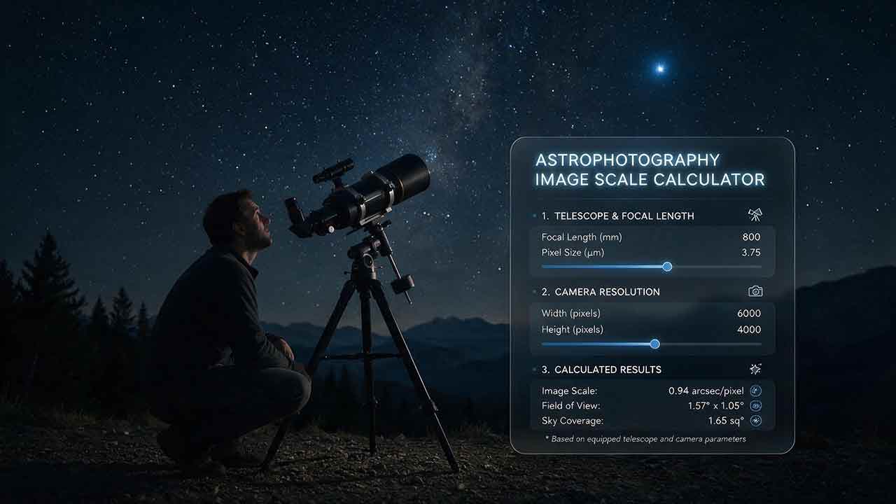
Astrophotography Image Scale Calculator
An Astrophotography Image Scale Calculator converts camera pixel size and effective focal length into arcseconds per pixel. For a small pixel near the optical axis of an approximately rectilinear imaging system, use 206.265 × pixel size in microns ÷ focal length in millimeters. The result shows how much sky one native pixel records and helps compare camera–telescope combinations.
Key Takeaways
- Image scale is approximately 206.265 × pixel size ÷ effective focal length.
- A smaller arcseconds-per-pixel value means finer detector sampling, not automatically higher resolved detail.
- Compare image scale with stellar FWHM measured from native-resolution, minimally processed data.
- About two or more samples across a point-spread-function FWHM is a useful reference in many contexts, not a universal equipment rule.
- Reducers, amplifiers, binning, resampling, distortion, and realized optical spacing can change the scale reported in an actual image.
This guide explains how to calculate image scale, choose the correct inputs, interpret sampling without confusing it with resolution, measure representative stellar FWHM, and verify the realized scale with a plate-solved image.
Method note: Image-scale values were calculated from the stated small-angle formula and rounded to two decimal places using conventional half-up rounding. Sampling-ratio values were calculated as delivered FWHM divided by image scale and rounded to one decimal place using the same method. Both tables and all worked examples were checked in a separate calculation pass. They are mathematical analyses rather than field tests of a particular camera, telescope, mount, or observing site. Statements about delivered image quality should be verified with native-resolution, minimally processed data from the actual imaging system.
How Does the Astrophotography Image Scale Calculator Work?
For a small pixel near the optical axis of an approximately rectilinear imaging system:
Image scale (arcsec/pixel)
≈ 206.265 × pixel size (µm)
÷ effective focal length (mm)
For a camera with 3.76µm pixels on an 800mm optical system:
206.265 × 3.76 ÷ 800
= 0.97 arcseconds per pixel
One native pixel therefore spans approximately 0.97 arcseconds on the sky near the optical axis under the assumptions of the formula.
The NASA Planetary Data System includes arcsec/pixel among its supported angular pixel-resolution units. NASA defines an arcsecond as 1/3,600 of a degree.
Why Is the Constant 206.265?
One radian contains approximately 206,264.806 arcseconds.
For a pixel of physical width (p) and an effective focal length (f), the small-angle approximation gives:
Angular width in radians
≈ pixel width ÷ focal length
When pixel size is entered in microns and focal length in millimeters:
Image scale
≈ 206,264.806 × (pixel size ÷ 1,000)
÷ focal length

≈ 206.265 × pixel size
÷ focal length
Astropy’s pixel- and plate-scale equivalencies document conversions among angular units, focal-plane distances, and detector pixels.
What Values Should You Enter?
Enter two required values:
- Pixel size in microns: Use the native pixel pitch published by the camera manufacturer.
- Effective focal length in millimeters: Use the focal length of the complete optical system in its imaging configuration.
Use effective focal length rather than the telescope’s printed nominal focal length when the imaging train includes:
- a focal reducer;
- an optical corrector that changes magnification;
- a Barlow lens;
- a telecentric amplifier;
- an extender;
- spacing-sensitive reduction or amplification.
For a zoom camera lens, use the focal length selected for the exposure.
What If the Detector Has Non-Square Pixels?
Most modern astronomy cameras have square pixels, but the formula can be applied separately to each axis when horizontal and vertical pixel pitches differ:
Horizontal image scale
≈ 206.265 × horizontal pixel pitch
÷ effective focal length

Vertical image scale
≈ 206.265 × vertical pixel pitch
÷ effective focal length
Do not average unequal axis values unless a single representative number is genuinely appropriate for the task.
Input Limits
Before trusting the result, confirm that:
- pixel size is a positive numeric value in microns;
- effective focal length is a positive numeric value in millimeters;
- sensor width or diagonal was not entered as pixel size;
- focal ratio was not entered in place of focal length;
- reducer or amplifier factors were applied only once;
- native pixel pitch is used unless binning is calculated separately;
- a crop or region of interest is not mistaken for binning;
- a resized image is not assumed to preserve native detector sampling;
- horizontal and vertical pitches are treated separately when pixels are not square.
Do not rely on a result produced from blank, zero, negative, nonnumeric, or incorrectly labeled input.
Exact On-Axis Pixel-Angle Formula
For an on-axis pixel in an ideal rectilinear optical system, angular width can be written without the small-angle approximation as:
On-axis pixel angle
= 2 × arctan(
    pixel width
    ÷ (2 × effective focal length)
  )
Pixel width and focal length must use the same physical units.
For ordinary astronomy-camera pixels and telescope focal lengths, pixel width is extremely small relative to focal length. The result is therefore effectively the same as:
Image scale
≈ 206.265 × pixel size in microns
÷ effective focal length in millimeters
Away from the optical axis, local angular scale can differ because of projection geometry or optical distortion. Use a calibrated World Coordinate System when position-dependent scale matters.
Image Scale, Plate Scale, Resolution, and Field of View Are Different
These terms describe related but distinct properties.
| Term | Meaning | Common unit |
|---|---|---|
| Image scale or pixel scale | Angular sky width recorded by one image pixel | arcsec/pixel |
| Classical plate scale | Angular sky width per physical distance in the focal plane | arcsec/mm |
| Instrument plate scale | Some observatory documentation uses this term for angular width per detector pixel | arcsec/pixel |
| Field of view | Total angular width and height recorded by the sensor | degrees or arcminutes |
| Resolution | Smallest detail the complete system can distinguish under stated conditions | arcseconds |
| Sampling | Number of detector samples used to represent delivered image detail | pixels per FWHM or another PSF-width measure |
Terminology is not perfectly uniform across observatories and software. This guide uses image scale for arcseconds per pixel and classical plate scale for arcseconds per millimeter unless a cited source uses another convention.
For example, the HST STIS documentation reports instrument plate scales in arcseconds per pixel and lists separate values for the detector axes.
Image Scale Does Not Equal Resolution
A system recording 0.50 arcsec/pixel does not automatically resolve 0.50-arcsecond detail.
Delivered image quality may instead be limited by:
- atmospheric turbulence;
- telescope diffraction;
- optical aberrations;
- focus accuracy;
- guiding and tracking;
- wind or vibration;
- filter wavelength;
- target signal-to-noise ratio;
- processing choices.
The European Southern Observatory distinguishes atmospheric seeing from image quality delivered in the focal plane. For equipment matching, measured stellar FWHM from the complete imaging system is generally more informative than a generic seeing forecast.
How Is Field of View Related to Image Scale?
For a narrow or moderate field:
Field width in arcseconds
≈ horizontal pixel count × horizontal image scale

Field height in arcseconds
≈ vertical pixel count × vertical image scale
Divide arcseconds by 60 for arcminutes or by 3,600 for degrees.
For an ideal rectilinear optical system, field of view along one sensor dimension is:
Field of view
= 2 × arctan(
    sensor dimension
    ÷ (2 × effective focal length)
  )
Sensor dimension and focal length must use the same units.
This geometric formula does not model fisheye projection, strong barrel or pincushion distortion, anamorphic behavior, or local scale changes across a distorted field. A plate-solved native-resolution image is preferable when realized field geometry matters.
Use a Telescope Field of View Calculator when the primary question is whether the complete target fits on the sensor.
Image Scale by Pixel Size and Focal Length
The following original comparison table shows image scale for four representative pixel pitches and seven focal lengths.
Assumptions:
- square native pixels;
- 1×1 capture;
- no resampling;
- stated effective focal length;
- scale evaluated near the optical axis.
| Pixel size | 250mm | 400mm | 600mm | 800mm | 1,000mm | 1,500mm | 2,000mm |
|---|---|---|---|---|---|---|---|
| 2.40µm | 1.98″/px | 1.24″/px | 0.83″/px | 0.62″/px | 0.50″/px | 0.33″/px | 0.25″/px |
| 3.76µm | 3.10″/px | 1.94″/px | 1.29″/px | 0.97″/px | 0.78″/px | 0.52″/px | 0.39″/px |
| 4.63µm | 3.82″/px | 2.39″/px | 1.59″/px | 1.19″/px | 0.96″/px | 0.64″/px | 0.48″/px |
| 5.94µm | 4.90″/px | 3.06″/px | 2.04″/px | 1.53″/px | 1.23″/px | 0.82″/px | 0.61″/px |
The table does not rank cameras or telescopes. It shows two geometric relationships:
- smaller pixels produce a finer scale at the same focal length;
- longer focal length produces a finer scale with the same camera.
Whether that finer scale is useful depends on the image delivered by the entire system.
How Should You Interpret the Result?
There is no universally best image scale. A useful value matches three things:
- detector sampling geometry;
- image quality delivered by the complete system;
- angular detail that matters in the target.
The Scale–Quality–Target Check
Original framework: The Scale–Quality–Target Check was created for this guide to organize image-scale decisions. It is an editorial planning framework, not a formal observatory standard or universal purchasing rule.
1. Scale: What Does Each Pixel Cover?
Calculate native image scale:
Scale
= 206.265 × pixel size
÷ effective focal length
This is a detector-geometry result. It does not grade the camera, telescope, mount, or final image.
2. Quality: How Large Are Stars in Real Data?
Measure the delivered FWHM of unsaturated stars in representative native-resolution data.
Then calculate:
Sampling ratio
= delivered stellar FWHM (arcsec)
÷ image scale (arcsec/pixel)
For a delivered FWHM of 2.4 arcseconds at 0.97 arcsec/pixel:
2.4 ÷ 0.97
= 2.47 pixels per FWHM
The STScI NIRCam documentation describes FWHM greater than about two pixels as Nyquist sampling or better for specified JWST modes and notes that undersampled modes can benefit from subpixel dithering.
That instrument-specific documentation supports two pixels as a useful sampling reference. It does not establish a universal boundary for every ground-based telescope, PSF shape, target, wavelength, or measurement task.
3. Target: Is the Sampling Useful for the Subject?
For a target feature of angular width (A):
Feature width in pixels
= feature width in arcseconds
÷ image scale
A 12-arcsecond feature at 0.8 arcsec/pixel spans approximately 15 pixels.
That arithmetic describes how the feature is sampled. It does not prove that all internal structure will be resolved, because seeing, optics, guiding, focus, and signal may remove smaller detail before it reaches the final image.
Use the framework in this order:
Calculate scale
→ measure delivered quality
→ evaluate target detail
How Should Representative Stellar FWHM Be Measured?
For the cleanest equipment comparison, prefer several calibrated native-resolution subframes measured before registration.
Use:
- unsaturated stars;
- several stars rather than one selected star;
- a representative region of the field;
- the normal filter and exposure duration;
- the normal focus and guiding workflow;
- images that have not been sharpened, deconvolved, drizzled, resized, upscaled, downsampled, or subjected to star-size reduction.
Report a median or similarly robust representative value. State whether the measurement is in pixels or arcseconds.
If individual subframes are too noisy for reliable measurements, a consistently processed native-scale linear stack can be used when it:
- retains the native output scale;
- is not drizzled or resized;
- has not been sharpened or deconvolved;
- uses the same registration and integration method across all compared datasets.
Registration interpolation and stacking can slightly change the measured point-spread function. Do not compare a single calibrated subframe from one setup with a heavily registered or resampled stack from another as though the measurements were equivalent.
If FWHM is measured in arcseconds:
Pixels per FWHM
= FWHM in arcseconds
÷ image scale in arcsec/pixel
If FWHM is measured directly in native pixels:
Pixels per FWHM
= measured FWHM in native pixels
Practical Sampling Bands for Seeing-Limited Deep-Sky Imaging
The following bands are an original planning aid for conventional long-exposure, seeing-limited deep-sky imaging with approximately star-like point-spread functions.
They are not universal pass-or-fail standards and should not be applied unchanged to:
- diffraction-limited imaging;
- adaptive-optics data;
- lucky imaging;
- lunar or planetary video;
- specialized astrometry or photometry;
- strongly non-Gaussian point-spread functions;
- data reconstructed from planned subpixel dithers.
| Pixels across delivered FWHM | Planning interpretation | Main consideration |
|---|---|---|
| Below 1.5 | Strongly coarse native sampling | Shape and centroid information may be limited without adequate dithering or modeling |
| 1.5–2.0 | Near-critical native sampling | Can work for wide fields; subpixel dithering becomes especially valuable |
| 2.0–3.5 | Balanced planning range | Often provides useful sampling without extreme file-size or guiding demands |
| 3.5–5.0 | Fine sampling | Most useful when tracking, focus, optics, and signal support the added samples |
| Above 5.0 | Strongly fine sampling for the measured FWHM | Additional pixels may describe the same delivered blur rather than reveal new detail |
The word balanced refers only to this guide’s sampling framework. It does not certify an equipment combination or predict final image quality.
Sampling-Ratio Reference Table
Each cell is calculated as:
Pixels per FWHM
= delivered FWHM in arcseconds
÷ image scale in arcsec/pixel
Values are rounded to one decimal place using conventional half-up rounding. For example, 1.5 ÷ 1.2 equals 1.25 and is displayed as 1.3.
| Delivered FWHM | 0.4″/px | 0.6″/px | 0.8″/px | 1.0″/px | 1.2″/px | 1.5″/px | 2.0″/px |
|---|---|---|---|---|---|---|---|
| 1.5″ | 3.8 px | 2.5 px | 1.9 px | 1.5 px | 1.3 px | 1.0 px | 0.8 px |
| 2.0″ | 5.0 px | 3.3 px | 2.5 px | 2.0 px | 1.7 px | 1.3 px | 1.0 px |
| 2.5″ | 6.3 px | 4.2 px | 3.1 px | 2.5 px | 2.1 px | 1.7 px | 1.3 px |
| 3.0″ | 7.5 px | 5.0 px | 3.8 px | 3.0 px | 2.5 px | 2.0 px | 1.5 px |
At 0.4 arcsec/pixel, a 2.0-arcsecond stellar profile covers five pixels. The detector is sampling that delivered profile finely, but the calculation does not make the atmosphere or optical system deliver 0.4-arcsecond resolution.
Calculation-Based Examples
These examples show formula results, not hands-on equipment tests.
Example 1: 3.76µm Pixels at 800mm
Image scale
= 206.265 × 3.76 ÷ 800
= 0.97 arcsec/pixel
Suppose minimally processed native-resolution data show a median stellar FWHM of 2.4 arcseconds:
Sampling ratio
= 2.4 ÷ 0.97
= 2.47 pixels per FWHM
Under the original planning bands used in this guide, 2.47 pixels per delivered FWHM falls within the stated balanced range.
This describes sampling only. It does not independently grade the telescope, camera, mount, target selection, or final image quality.
Example 2: Doubling Focal Length Without Improving Delivered FWHM
Use the same 3.76µm camera at 1,600mm:
Image scale
= 206.265 × 3.76 ÷ 1,600
= 0.48 arcsec/pixel
If delivered stellar FWHM remains 2.4 arcseconds:
Sampling ratio
= 2.4 ÷ 0.48
= 5.0 pixels per FWHM
The longer system records approximately twice as many pixels across the same delivered star width. It does not automatically double resolved detail.
Finer sampling may still assist registration, centroiding, carefully controlled deconvolution, or small-target presentation. It also places greater demands on focus, tracking, guiding, stability, and signal.
Example 3: 5.94µm Pixels at 400mm
Image scale
= 206.265 × 5.94 ÷ 400
= 3.06 arcsec/pixel
If delivered stellar FWHM is 2.4 arcseconds:
Sampling ratio
= 2.4 ÷ 3.06
= 0.78 pixels per FWHM
This is strongly coarse native sampling under the planning bands in this guide. Small stellar shapes and fine target structure may be poorly represented.
The combination can still suit:
- large nebulae;
- broad dust regions;
- survey-style coverage;
- modest output sizes;
- workflows using well-planned dithering.
How Should Different Astrophotographers Use Image Scale?
Wide-Field Deep-Sky Imaging
Prioritize:
- target fit;
- total field coverage;
- manageable tracking;
- acceptable rather than extreme sampling;
- reliable dithering.
A moderately coarse scale can be a rational tradeoff when the target spans a large area of sky.
Small-Galaxy and Planetary-Nebula Imaging
Prioritize:
- measured delivered FWHM;
- focus stability;
- mount performance;
- optical quality;
- target signal-to-noise ratio.
A finer scale is useful only when the system preserves corresponding angular information.
Lunar and Planetary Imaging
Image scale remains relevant, but the long-exposure seeing-limited bands in this guide should not be applied unchanged.
High-frame-rate lunar and planetary workflows also depend on:
- aperture;
- wavelength;
- diffraction;
- short-exposure seeing;
- frame selection;
- optical amplification;
- reconstruction method.
Use a Telescope Resolution Calculator when comparing image scale with diffraction and aperture.
Photometry and Astrometry
Very coarse or unstable stellar sampling can make centroid and aperture measurements more sensitive to pixel phase, undersampling, and point-spread-function changes.
Measurement precision also depends on:
- signal-to-noise ratio;
- saturation and detector linearity;
- flat-field quality;
- intrapixel response;
- crowding;
- tracking;
- detector stability;
- the fitting or aperture method.
Do not select an astrometric or photometric setup from image scale alone. Validate it with representative data and the intended measurement pipeline.
Does a Finer Image Scale Always Produce More Detail?
No. Finer sampling records more pixels per angular unit, but resolved detail remains limited by the complete imaging chain.
Advantages of a Finer Scale
- More samples across a star or small structure
- Greater flexibility for registration
- Potentially improved centroid measurements
- More room for controlled deconvolution
- Less obvious pixelation at large display sizes
- Better presentation of small targets when conditions support it
Tradeoffs of a Finer Scale
- More demanding tracking and guiding
- Greater sensitivity to wind and focus drift
- More pixels describing the same blurred signal
- Larger files and longer processing
- Smaller field of view when achieved through longer focal length
- No guaranteed resolution gain
Advantages of a Coarser Scale
- Wider field when produced by shorter focal length
- More forgiving tracking at the displayed pixel level
- A point-spread function may cover fewer native pixels
- Potentially higher signal per sampled pixel in some larger-pixel or binned configurations
- Smaller files and faster processing
- Practical coverage for large targets
A coarser image scale does not by itself guarantee more total captured photons or a better signal-to-noise ratio. Photon collection also depends on aperture, focal ratio, throughput, exposure time, target surface brightness, pixel area, read noise, and processing.
Tradeoffs of a Coarser Scale
- Fewer samples across the stellar profile
- Greater risk of blocky star shapes
- Less centroid information
- Reduced representation of small structures
- No ability to reconstruct information that was never sampled
How Do Reducers, Amplifiers, and Binning Change Image Scale?
Focal Reducers
A reducer shortens effective focal length and increases arcseconds per pixel.
Example:
Native focal length: 1,000mm
Reducer factor: 0.8×
Effective focal length: 800mm
For 3.76µm pixels:
At 1,000mm: 0.78″/pixel
At 800mm:   0.97″/pixel
The reduced system records a wider field and a coarser image scale.
Actual reduction can depend on optical spacing, so a plate-solved effective focal length may differ from the label.
Barlow Lenses and Extenders
A nominal 2× amplifier approximately doubles focal length and halves arcseconds per pixel:
800mm at 0.97″/pixel
→ 1,600mm at about 0.48″/pixel
Actual amplification can depend on spacing and optical design.
Hardware or Capture Binning
For true 2×2 spatial binning, two native pixel intervals are combined along each image axis.
Geometrically:
Effective sampling interval
= native pixel pitch × 2

Effective image scale
= native image scale × 2
A native scale of 0.75 arcsec/pixel therefore becomes approximately 1.50 arcsec per binned output pixel.
This relationship assumes a regular 2×2 combination. Read-noise behavior, summing versus averaging, Bayer-pattern handling, bit depth, and metadata reporting vary by camera and software. Confirm what the selected binning mode actually does.
Software Resizing and Resampling
Resizing changes the displayed output scale but does not change the angular information originally sampled by the detector.
Upscaling cannot restore detail that was never recorded. Downsampling can improve presentation and apparent signal-to-noise per output pixel, but it does not change the original optical resolution.
How Can You Verify the Actual Image Scale?
A practical verification method is to plate-solve a native-resolution image and inspect its celestial World Coordinate System, or WCS.
Treat a reference-pixel value as a local or representative scale rather than proof that every part of a distorted field has exactly the same scale.
Astropy’s proj_plane_pixel_scales function returns projection-plane pixel scales along the image axes at the WCS reference-pixel location. Its documentation states that the function does not include distortions caused by the nonlinear celestial projection.
For a narrow, well-corrected field, the reference scale is often a useful summary. For a wide or distorted field, inspect the full WCS transformation or compare local sky-coordinate separations at several image positions.
Why Might Plate Solving Report a Different Scale?
Possible reasons include:
- nominal focal length differs from realized focal length;
- reducer spacing changes magnification;
- a Barlow operates at a different factor from its label;
- the image was binned;
- the file was resized, drizzled, or resampled;
- incorrect pixel-size data were entered;
- a crop was mistaken for binning;
- distortion changes local scale;
- horizontal and vertical scales differ;
- metadata describe a processed image rather than native capture geometry.
Deriving an Effective Focal Length from Measured Scale
For a native-resolution image with known pixel pitch, rearrange the image-scale formula:
Effective focal length (mm)
= 206.265 × pixel size (µm)
÷ measured image scale (arcsec/pixel)
For 3.76µm pixels and a measured scale of 1.02 arcsec/pixel:
206.265 × 3.76 ÷ 1.02
= approximately 760mm
This is the effective focal length corresponding to the measured local or representative image scale.
Use an axis-appropriate value when horizontal and vertical scales differ. An averaged value is reasonable only when that choice matches the purpose of the calculation.
Significant distortion, unequal axis scales, non-square pixels, binning, drizzle, or resizing can make one focal-length value an incomplete description of the processed image.
Step-by-Step Image-Scale Workflow
Step 1: Confirm Native Pixel Size
Use the camera manufacturer’s published pixel pitch.
Do not substitute sensor width, diagonal, total megapixels, or output dimensions.
Step 2: Determine Effective Focal Length
Include reducers, amplifiers, and other optics that change image magnification.
Use a reliable plate-solved value when available.
Step 3: Calculate Native Image Scale
206.265 × pixel size ÷ focal length
Retain the unrounded value for internal calculations and display a sensible number of decimal places.
Step 4: Measure Representative FWHM
Prefer several calibrated native-resolution subframes with unsaturated stars.
Use a consistently processed native-scale linear stack only when individual subframes are too noisy for reliable measurement.
Step 5: Calculate Pixels per FWHM
Delivered FWHM in arcseconds
÷ image scale in arcsec/pixel
A native-pixel FWHM measurement already expresses this sampling ratio.
Step 6: Check the Intended Target
Confirm that:
- the complete object fits within the field;
- useful small-scale structure receives meaningful sampling;
- the mount and focus system can support the chosen scale.
Step 7: Verify with a Plate-Solved Exposure
Compare calculated image scale with the WCS value from a native-resolution frame.
For a distorted field, examine more than one location and do not assume one scale represents every pixel.
Common Image-Scale Mistakes
Using Sensor Size Instead of Pixel Size
Image scale requires one pixel’s physical pitch. Sensor dimensions determine total field of view.
Using Aperture Instead of Focal Length
Aperture affects diffraction and light collection. Focal length controls geometric image scale.
Ignoring a Reducer or Amplifier
Use the effective focal length of the complete imaging train.
Treating Image Scale as Guaranteed Resolution
A calculation of 0.5 arcsec/pixel does not guarantee 0.5-arcsecond resolved detail.
Classifying Sampling from a Weather Seeing Number Alone
Whenever possible, use FWHM measured from the image delivered by the actual telescope, camera, filter, focus, tracking, and exposure workflow.
Confusing Crop Mode with Binning
Cropping removes outer pixels without changing native angular scale. True spatial binning combines adjacent sampling intervals.
Measuring a Resized File
A resized output may no longer represent native detector sampling. Use a native-resolution frame for verification.
Troubleshooting
| Problem | Possible cause | Practical response |
|---|---|---|
| Plate-solved scale differs from the calculation | Effective focal length, pixel size, binning, or processing history is wrong | Check optical spacing, camera specifications, image dimensions, and metadata |
| Stars look blocky | Coarse native sampling or aggressive enlargement | Dither, use a finer native scale, or reduce output enlargement |
| Stars remain large at a fine scale | Seeing, focus, guiding, vibration, or optics dominate | Measure representative FWHM and diagnose the delivered image quality |
| A longer focal length adds no visible detail | Seeing, focus, guiding, optics, signal-to-noise ratio, target structure, or already-fine sampling may limit the result | Compare matched integrations, FWHM, guiding error, focus, and optical quality before blaming sampling alone |
| Field of view is smaller than expected | Realized focal length is longer than assumed | Plate-solve a native image and recalculate |
| Horizontal and vertical scales differ | Non-square pixels, resampling, axis distortion, or WCS geometry | Inspect both WCS axis scales and the processing history |
| Binned images show an unexpected scale | Software uses a different binning, averaging, or output convention | Verify capture mode, native dimensions, and metadata |
| Calculator output is implausible | Micron and millimeter units were mixed | Recheck units and input labels |
| Guiding appears worse after changing cameras | The new imaging scale is finer | Compare guiding error in arcseconds rather than guide-camera pixels alone |
Equipment-Matching Checklist
Before selecting or changing a camera–telescope combination:
- Confirm native pixel pitch.
- Confirm effective imaging focal length.
- Include reducer or amplifier factors.
- Calculate native arcseconds per pixel.
- Estimate total field of view separately.
- Measure stellar FWHM from representative native-resolution data.
- Calculate pixels per delivered FWHM.
- Consider the target’s angular size and useful structure.
- Compare guiding error with image scale.
- Account for intended binning or downsampling.
- Verify realized scale with a plate-solved image.
- Inspect multiple image positions when distortion matters.
- Avoid treating one sampling band as a universal buying rule.
Use a Focal Ratio Calculator when evaluating focal speed, a Telescope Magnification Calculator for visual configurations, and the Rule of 500 Calculator for Milky Way Photography for untracked wide-field exposure planning.
Practical Conclusion
The Astrophotography Image Scale Calculator answers one geometric question:
How much sky does each native pixel record?
Use:
Image scale
≈ 206.265 × pixel size in microns
÷ effective focal length in millimeters
Then measure the stellar FWHM delivered by representative native-resolution exposures and evaluate whether the target benefits from that sampling.
Calculate scale
→ measure image quality
→ match the target
Wide-field imagers should prioritize target coverage and stable acquisition. Small-target imagers should choose finer sampling only when seeing, focus, optics, guiding, and signal support it. Lunar and planetary imagers should combine image scale with wavelength, diffraction, aperture, and short-exposure technique.
Frequently Asked Questions
Is a Smaller Arcseconds-per-Pixel Value Always Better?
No. It means finer sampling, but real detail may still be limited by seeing, focus, tracking, optics, and signal-to-noise ratio.
What Image Scale Should I Use for Deep-Sky Astrophotography?
Measure delivered stellar FWHM and compare it with image scale. About two to several pixels per FWHM can be a useful planning range for conventional seeing-limited deep-sky imaging, but it is not a universal standard.
Does Crop Factor Affect Image Scale?
Crop factor is not an input to the native image-scale formula. Native image scale depends on physical pixel pitch and effective focal length.
A smaller sensor with the same pixel pitch records a narrower total field but retains the same native arcseconds per pixel. If the smaller sensor also has a different pixel pitch, image scale changes because of the pixel pitch—not because of crop factor itself.
Does 2×2 Binning Double Arcseconds per Output Pixel?
For a true 2×2 spatial combination, yes. The output sampling interval doubles along each axis, and each output sample covers four times the angular area. Noise, summing, color, and metadata behavior depend on implementation.
Why Does Plate Solving Report a Different Focal Length?
Nominal and realized focal lengths can differ because of optical spacing, reducer or amplifier behavior, binning, distortion, and processing. Check a native-resolution image and treat the WCS scale as local or representative when distortion is present.
Can Drizzle Fix Undersampling?
Planned subpixel dithering can improve effective PSF sampling when exposures contain useful fractional-pixel offsets. The STScI dithering overview explains how dithering can improve sampling. Drizzle cannot guarantee recovery of information absent from the observations or correct poor focus, tracking, or signal.
Sources
NASA Planetary Data System — Angular Pixel-Resolution Units
Supported angular pixel-resolution units, including arcseconds per pixel. Accessed August 1, 2026.NASA Science — Universe Glossary
Definition of an arcsecond as 1/3,600 of a degree. Accessed August 1, 2026.Astropy — Pixel and Plate Scale Equivalencies
Software documentation for conversions among detector pixels, focal-plane distances, and angular scales. Accessed August 1, 2026.European Southern Observatory — Observing Conditions Definitions
Distinction between atmospheric seeing and delivered focal-plane image quality measured by stellar FWHM. Accessed August 1, 2026.STScI — NIRCam Point-Spread Functions
Instrument-specific documentation on PSF FWHM, Nyquist sampling, undersampling, and subpixel dithering. Accessed August 1, 2026.STScI — JWST Dithering Overview
How dithering can support improved point-spread-function sampling. Accessed August 1, 2026.Astropy —
proj_plane_pixel_scales
Projection-plane pixel scales at the WCS reference pixel and limitations involving nonlinear celestial projections. Accessed August 1, 2026.Astropy — World Coordinate System
Pixel-to-world-coordinate transformations using celestial WCS information. Accessed August 1, 2026.HST User Documentation — STIS Image-Mode Geometric Distortion
Measured detector-axis scales, geometric distortion, and rectified-image plate scales. Accessed August 1, 2026.HST User Documentation — STIS Plate Scales
Observatory use of plate scale in arcseconds per detector pixel. Accessed August 1, 2026.
More from Astrophotography Planning Tools
Astrophotography Storage Calculator
This guide explains how to estimate storage for astrophotography capture, processing, and backup without relying on misleading megapixel shortcuts. It compares measured-file, uncompressed-array, and bitrate methods; distinguishes mean, median, high-percentile, and maximum file-size statistics; and explains decimal versus binary storage units. Readers learn how FITS headers, padding, HDUs, RAW compression, calibration frames, RGB conversion, drizzle, mosaics, caches, and temporary files affect project size. Original planning tools include the Four-Bucket Storage Ledger, the Capture–Process–Protect Check, and a clearly defined storage expansion ratio. Worked examples show how to calculate peak logical data, project-relative headroom, complete-copy footprint, media count, write rate, and transfer time. The article also covers integrity verification, backup limitations, retention decisions, and troubleshooting. It is designed to help astrophotographers build realistic capacity plans for single sessions, multi-night projects, planetary video, star trails, and long-term archives.
Star Trail Exposure Calculator
This guide explains how to calculate star-trail exposure time from Earth’s sidereal rotation, stellar declination, and local image scale. It distinguishes polar sweep, declination-adjusted sky-path length, projected pixel length, recorded sweep, missing sweep, and the full start-to-end span of a stacked sequence. Original tables compare trail lengths at several declinations, quantify one-second frame gaps at different image scales, and show how recorded time, gap time, duty cycle, and sequence sweep relate. The Trail–Frame–Sequence Check provides a practical framework for separating celestial geometry, per-frame reliability, and sequence continuity. Worked examples also address the celestial-pole edge case, local WCS-based pixel movement, frame-count limits, long-exposure noise reduction, and the difference between a single exposure and stacked frames. Readers can use the article to plan smoother trails, avoid misleading sequence calculations, and verify expected motion with native-resolution test images.
Camera Field of View Calculator
This guide explains how to calculate horizontal, vertical, and diagonal camera field of view from the recorded active sensor dimensions and effective focal length. It distinguishes physical focal length from crop-factor comparisons, shows why aspect ratio and target rotation affect framing, and provides independently calculated reference tables for common sensor sizes and focal lengths. The original Frame Envelope Check separates ideal frame geometry, the target envelope, and the usable frame retained after dithering, registration, distortion correction, and cropping. Worked examples demonstrate target occupancy, maximum permitted focal length, rotated bounding boxes, and mosaic panel counts with overlap. The article also explains radians versus degrees, crop and stabilization modes, focus breathing, rectilinear versus fisheye projection, and plate-solving verification through a celestial WCS. Readers can use the formulas, margin budget, troubleshooting table, and framing checklist to plan wide-field compositions, small-target imaging, or mosaics without treating a mathematical edge-to-edge fit as a guaranteed final frame.
Explore More Topics
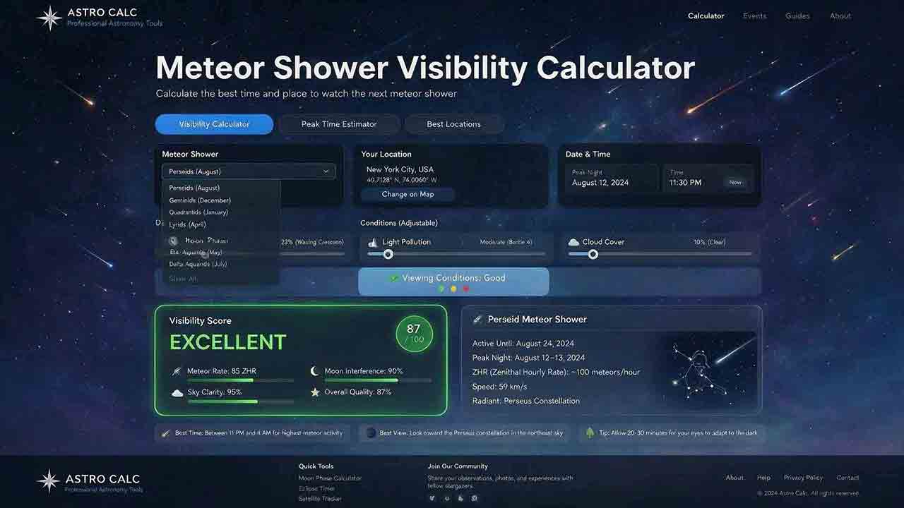
Meteor Shower Visibility Calculator
This guide explains how to use a meteor shower visibility calculator to identify a locally favorable observing window instead of relying only on a published peak time or Zenithal Hourly Rate. It covers activity periods, radiant altitude, astronomical darkness, Moon timing, weather, limiting magnitude, population index, and the distinction between named-shower members, sporadic meteors, and meteors from overlapping showers. The article introduces two original planning tools: the Five-Layer Meteor Test and the Meteor Opportunity Window, which calculates the overlap between activity, radiant, darkness, Moon, weather, and session constraints. A reproducible cross-midnight example compares illustrative 20° and 40° radiant thresholds, producing windows of 2 hours 20 minutes and 1 hour 40 minutes. Practical guidance addresses moonlight, viewing direction, dark adaptation, calculator disagreements, troubleshooting, and responsible site selection, supported by NASA, IMO, AMS, and U.S. Naval Observatory sources.
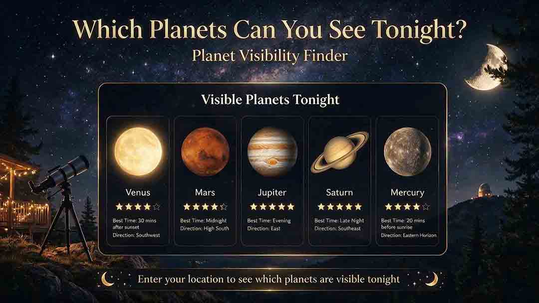
Planet Visibility Finder: Which Planets Can You See Tonight?
This guide explains how to use a planet visibility finder to decide which planets are realistically observable for a selected date, time, and location. It shows why an object being above the horizon does not guarantee visibility and explains the roles of altitude, azimuth, apparent magnitude, solar elongation, twilight, moonlight, weather, and local obstructions. Readers learn which planets are normally visible without a telescope, how Mercury and Venus differ from the outer planets, and why two finders may produce different results. The article introduces an original Four-Gate Visibility Test covering position, solar light, detectability, and site timing, plus a reproducible Useful Viewing Window calculation. A hypothetical example compares a 1-hour-26-minute naked-eye window with an 18-minute higher-altitude telescope window. Practical troubleshooting, safety guidance, and NASA, USNO, and JPL sources support the planning method.
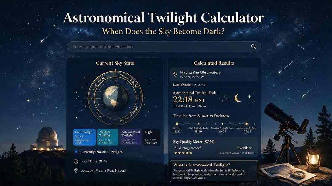
Astronomical Twilight Calculator: When Does the Sky Become Dark?
This guide explains how to use an astronomical twilight calculator to identify the end of evening astronomical twilight and the beginning of morning astronomical twilight for a selected date and location. It distinguishes sunset, civil dusk, nautical dusk, astronomical dusk, and the Sun-below-18° interval while clarifying that solar geometry does not guarantee a visibly dark sky. Readers learn how latitude, season, timezone, daylight-saving rules, moonlight, skyglow, clouds, haze, and high-latitude conditions affect practical planning. The article introduces two original tools: the Darkness Margin, which calculates how much of a session falls inside the Sun-below-18° interval, and a Task Threshold Matrix that matches observing goals to practical twilight stages. A worked cross-midnight example produces a 1-hour-48-minute dark interval. Troubleshooting guidance, planning checks, and authoritative USNO, NOAA, and National Park Service sources support the method.