Camera Field of View Calculator

Camera Field of View Calculator
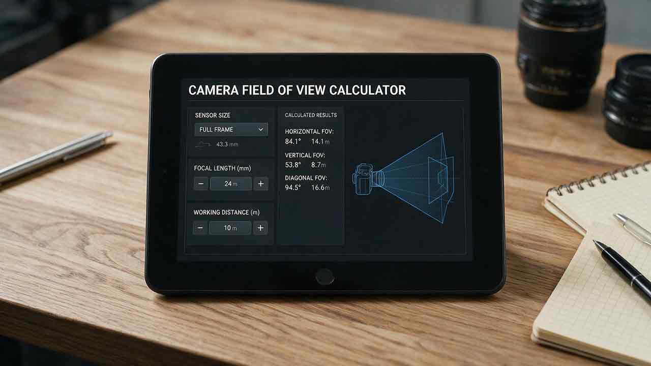
A Camera Field of View Calculator estimates how much sky a camera records from its active sensor dimensions and effective focal length. For an ideal rectilinear system, calculate each frame axis with 2 × arctan(sensor dimension ÷ (2 × focal length)). Use the recorded active area—not only a crop-factor label—and leave room for rotation, dithering, registration, distortion correction, and final cropping.
Key Takeaways
- Calculate horizontal, vertical, and diagonal field of view separately.
- Use the physical dimensions of the recorded active area and the effective focal length near infinity focus.
- Crop factor is a comparison shortcut; it is not required by the field-of-view formula.
- A target that fits mathematically may still be framed too tightly for rotation, dithering, stacking, or correction crops.
- Verify important compositions with a native-resolution, plate-solved image whenever possible.
The calculator’s core outputs are horizontal, vertical, and diagonal field of view. The additional formulas in this guide can be used to estimate maximum focal length, target occupancy, rotation, framing margin, and mosaic coverage.
Method note: The field-of-view tables and worked examples in this guide were calculated from the stated rectilinear formulas and checked in a separate calculation pass. Displayed angles use conventional half-up rounding. The calculations are geometric planning analyses rather than hands-on tests of particular cameras, lenses, telescopes, or software. Realized framing should be verified when distortion, crop modes, image stabilization, optical spacing, stacking, or post-capture correction can alter the usable frame.
How Does the Camera Field of View Calculator Work?
For an ideal rectilinear imaging system focused at or near infinity:
Field of view
= 2 × arctan(
    sensor dimension
    ÷ (2 × effective focal length)
  )
Sensor dimension and focal length must use the same physical unit. Millimeters are normally the most convenient choice.
Calculate each frame axis separately:
Horizontal FOV
= 2 × arctan(
    sensor width
    ÷ (2 × focal length)
  )

Vertical FOV
= 2 × arctan(
    sensor height
    ÷ (2 × focal length)
  )

Diagonal FOV
= 2 × arctan(
    sensor diagonal
    ÷ (2 × focal length)
  )
The sensor diagonal is:
Sensor diagonal
= √(sensor width² + sensor height²)
Canon’s official Angle of View Calculator likewise treats horizontal, vertical, and diagonal angle of view as separate values based on image dimensions and focal length.
Diagonal FOV is useful for broad format comparisons and discussions of circular image coverage. It should not be the sole target-fit test for a rectangular sensor, because a target can fit within the diagonal angle while exceeding the horizontal or vertical frame boundary.
Angle Units
The formulas in this guide display field of view in degrees.
Most programming-language trigonometric functions use radians. When implementing the calculation:
FOV in degrees
= 2 × arctan(
    sensor dimension
    ÷ (2 × focal length)
  )
× 180 ÷ π
When a required field of view is entered in degrees:
Maximum focal length
= sensor dimension
÷ [
    2 × tan(
      required FOV in degrees
      × π ÷ 180
      ÷ 2
    )
  ]
For target-rotation calculations, convert the rotation angle to radians before using sin() or cos() unless the software is explicitly operating in degree mode.
Example: 24mm Lens on Full Frame
For a 36mm × 24mm active image area:
Horizontal FOV
= 2 × arctan(36 ÷ 48)
= 73.7°

Vertical FOV
= 2 × arctan(24 ÷ 48)
= 53.1°
The calculated frame is approximately:
73.7° × 53.1°
This describes ideal rectilinear geometry before accounting for lens distortion, in-camera correction, stabilization crops, stacking loss, or another reduction in active image area.
What Does Camera Field of View Mean?
Field of view is the angular width and height of the scene recorded by the active image area.
In this guide, field of view means the angular field recorded at astronomical or effectively infinite focus. Camera manufacturers may call the same quantity angle of view. It is expressed in degrees rather than as the linear width of a scene at a finite subject distance.
NASA defines a telescope’s field of view as its viewing area expressed in degrees, arcminutes, or arcseconds. Camera fields are commonly broad enough to express in degrees, while small telescope fields and celestial details are often expressed in arcminutes or arcseconds.
Which Inputs Should You Enter?
Use three values:
- Active sensor width
- Active sensor height
- Effective focal length
Do not substitute:
- megapixel count;
- pixel pitch;
- aperture;
- focal ratio;
- sensor diagonal alone when horizontal and vertical framing matter;
- 35mm-equivalent focal length combined with the original cropped-sensor dimensions;
- the complete zoom range instead of the selected focal length.
Use the Recorded Active Area
Published sensor dimensions may describe the physical sensor rather than every pixel used in the selected recording mode.
The recorded active area can be reduced by:
- aspect-ratio modes;
- raw or JPEG crops;
- video readout modes;
- high-frame-rate crops;
- electronic stabilization;
- optical-black rows or columns;
- distortion correction;
- computational capture modes.
Use the dimensions corresponding to the actual recorded image area whenever they are known.
Use Effective Focal Length Near Infinity Focus
For astronomical subjects, use the focal length realized near infinity focus.
Some photographic lenses change their angle of view as focus position changes. A field measurement made from a close indoor subject may therefore differ from the night-sky frame even when the lens reports the same nominal focal length.
Include any component that changes magnification:
- focal reducer;
- Barlow lens;
- telecentric amplifier;
- extender;
- spacing-sensitive reducer;
- optical corrector with a non-neutral magnification factor.
Input Limits
All dimensions must be positive numeric values.
Before using a result, confirm that:
- sensor dimensions and focal length use the same unit;
- width and height have not been reversed unintentionally;
- the selected active crop mode is known;
- reducer or amplifier factors are applied only once;
- the selected zoom focal length is used;
- a processed crop is not mistaken for the captured active area;
- blank, zero, negative, or nonnumeric values are treated as invalid.
A production calculator should return a clear input error rather than an apparently valid result when any required value is invalid.
How Can You Calculate the Maximum Focal Length?
Rearrange the field-of-view formula when the required angular field and sensor dimension are known:
Maximum focal length
= sensor dimension
÷ (2 × tan(required FOV ÷ 2))
When the required FOV is entered in degrees, convert it to radians inside the tangent calculation.
Calculate the maximum permitted focal length for both frame axes.
When the target must fit both horizontally and vertically, the smaller of the two axis-specific focal-length limits is the controlling value. The selected focal length must not exceed either limit.
For example:
Horizontal-axis limit: 269mm
Vertical-axis limit: 286mm
Controlling limit: 269mm
A focal length of 269mm or shorter satisfies both geometric requirements under the stated orientation and margin assumptions.
If the camera or target is rotated, calculate the rotated target width and height before deriving the two focal-length limits.
Why Is Crop Factor Not Enough?
Crop factor provides an approximate comparison with the diagonal field of a 36mm × 24mm full-frame sensor. Exact framing still depends on active sensor width, active sensor height, and aspect ratio.
A smaller sensor records a narrower portion of the same projected image when focal length remains unchanged. Nikon describes its full-frame FX format and smaller DX format in its DX and FX guide.
Equivalent Focal Length Is a Comparison
A 24mm lens on a 1.5× format is commonly described as providing a field similar to a 36mm lens on full frame:
24mm × 1.5
= 36mm equivalent
The physical lens remains a 24mm lens. The smaller sensor records less of the image circle.
For a direct field-of-view calculation, use:
actual focal length
+ active sensor dimensions
Do not use:
equivalent focal length
+ cropped sensor dimensions
That applies the format adjustment twice.
Aspect Ratio Can Change the Fit
Two sensors can have similar diagonal crop factors but different aspect ratios.
A 3:2 sensor and a 4:3 sensor may provide similar diagonal coverage while producing different horizontal and vertical fields. That difference matters when a target nearly fills one frame axis.
For astrophotography composition, physical width and height are therefore more informative than crop factor alone.
Common Active Sensor Dimensions
Format names are approximate categories, not guarantees that every camera records the same active dimensions. Use the specification for the actual camera and recording mode whenever possible.
| Representative format example | Documented sensor dimensions | Aspect ratio | First-party reference |
|---|---|---|---|
| Full-frame example | 36.0 × 24.0mm | 3:2 | Canon Angle of View Calculator |
| Nikon DX example | 23.5 × 15.6mm | about 3:2 | Nikon D7200 specifications |
| Canon APS-C example | 22.3 × 14.9mm | 3:2 | Canon EOS R100 specifications |
| Micro Four Thirds example | 17.3 × 13.0mm | 4:3 | OM System OM-5 specifications |
| 1-inch-type example | 13.2 × 8.8mm | 3:2 | Sony DSC-RX100 specifications |
The products in this table are documentation examples for physical dimensions. They were not tested, compared, ranked, or recommended for purchase.
Camera Field of View by Sensor Format and Focal Length
Each cell shows:
Horizontal FOV × Vertical FOV
Values assume an ideal rectilinear system and are rounded to one decimal place using conventional half-up rounding.
| Active sensor area | 14mm | 24mm | 35mm | 50mm | 85mm | 135mm | 200mm |
|---|---|---|---|---|---|---|---|
| Full frame, 36 × 24mm | 104.3° × 81.2° | 73.7° × 53.1° | 54.4° × 37.8° | 39.6° × 27.0° | 23.9° × 16.1° | 15.2° × 10.2° | 10.3° × 6.9° |
| APS-C, 23.5 × 15.6mm | 80.0° × 58.2° | 52.2° × 36.0° | 37.1° × 25.1° | 26.4° × 17.7° | 15.7° × 10.5° | 9.9° × 6.6° | 6.7° × 4.5° |
| Canon APS-C, 22.3 × 14.9mm | 77.1° × 56.0° | 49.8° × 34.5° | 35.3° × 24.0° | 25.1° × 16.9° | 14.9° × 10.0° | 9.4° × 6.3° | 6.4° × 4.3° |
| Micro Four Thirds, 17.3 × 13.0mm | 63.4° × 49.8° | 39.6° × 30.3° | 27.8° × 21.0° | 19.6° × 14.8° | 11.6° × 8.7° | 7.3° × 5.5° | 5.0° × 3.7° |
| 1-inch type, 13.2 × 8.8mm | 50.5° × 34.9° | 30.8° × 20.8° | 21.4° × 14.3° | 15.0° × 10.1° | 8.9° × 5.9° | 5.6° × 3.7° | 3.8° × 2.5° |
The table is a geometric planning reference, not a substitute for the camera’s recorded active-area specification or a plate-solved test frame.
The Frame Envelope Check
Original framework: The Frame Envelope Check was created for this guide to separate geometric field of view from practical target framing. It is an editorial planning framework, not an industry standard or a guarantee that a composition will succeed.
Use three checks in order:
Frame geometry
→ target envelope
→ realized capture
1. Frame Geometry: What Does the Camera Record?
Calculate horizontal and vertical field of view from the active sensor dimensions and effective focal length.
Do not begin with diagonal field alone. A target fails to fit when either its horizontal requirement or its vertical requirement exceeds the corresponding frame dimension.
2. Target Envelope: How Much Space Does the Target Need?
The target envelope includes:
- angular width and height;
- orientation relative to the sensor;
- faint outer structure that should remain;
- desired breathing room;
- dithering displacement;
- registration and stacking loss;
- planned final crop;
- mosaic overlap when applicable.
A mathematically exact edge-to-edge fit is usually fragile.
3. Realized Capture: What Does the System Deliver?
Confirm the real frame when the setup may be affected by:
- lens distortion;
- a fisheye or another non-rectilinear projection;
- reducer spacing;
- focus-dependent focal length;
- in-camera aspect-ratio crop;
- digital stabilization;
- video crop;
- distortion correction;
- stacking alignment;
- panorama projection;
- post-processing crop.
The final usable frame can be smaller than the ideal sensor calculation.
How Much Framing Margin Should You Leave?
There is no universal margin. The useful amount depends on the target, mount, dithering plan, stacking workflow, distortion, and intended crop.
The following original bands apply to a centered target after its intended orientation has been considered.
| Target occupancy on the limiting frame axis | Planning interpretation | Typical use |
|---|---|---|
| Below 50% | Context-heavy framing | Wide environmental composition or generous crop flexibility |
| 50–75% | Comfortable framing | General-purpose composition with useful margin |
| 75–85% | Tight but manageable | Detail-oriented framing with controlled acquisition |
| 85–95% | Fragile fit | Requires accurate rotation, centering, and crop planning |
| Above 95% | Edge-dependent fit | High clipping risk after dithering, stacking, correction, or alignment |
These are planning bands rather than quality scores. A deliberately wide composition can be preferable to a tight one, and a controlled mosaic may intentionally use detector edges.
Calculating Target Occupancy
For a modest or narrow rectilinear field:
Horizontal occupancy
≈ target width
÷ horizontal FOV
× 100%

Vertical occupancy
≈ target height
÷ vertical FOV
× 100%
Evaluate both axes separately.
Limiting occupancy
= max(
    horizontal occupancy,
    vertical occupancy
  )
The axis with the larger percentage controls the framing-risk classification.
For a centered, axis-aligned target:
Horizontal one-side margin
≈ (horizontal FOV − target width)
÷ 2

Vertical one-side margin
≈ (vertical FOV − target height)
÷ 2
After rotation, use the rotated target envelope rather than the original width and height.
For very wide fields, sky curvature and projection effects become important. Use a WCS-aware planning method rather than relying only on flat angular ratios.
Building a Framing-Margin Budget
Instead of choosing one unexplained margin, estimate the expected usable frame after acquisition and processing:
Usable frame
≈ geometric frame
− dithering loss
− registration loss
− correction crop
− planned final crop
Do not simply add percentage losses when they occur at different stages or on different sides of the frame.
A stronger method is to measure the common retained dimensions from a representative processed sequence. The target envelope should fit inside the estimated usable frame—not merely inside the original sensor field.
How Does Target Rotation Change the Required Frame?
A rectangular target can fit in one orientation and fail after rotation.
For a modest or narrow field represented in a local tangent plane:
θr
= rotation angle in degrees
× π ÷ 180

Rotated width
≈ |W × cos θr|
+ |H × sin θr|

Rotated height
≈ |W × sin θr|
+ |H × cos θr|
Where:
Wis target width;His target height;θris the rotation angle in radians.
The formula assumes that W and H are rectangular extents measured in the same local angular coordinate system.
Do not apply it directly to right-ascension and declination differences as if they were ordinary Cartesian width and height. Right-ascension separation represents a different physical sky distance at different declinations.
When deriving an envelope from celestial coordinates, use a sky-planning tool, WCS transformation, or local tangent-plane projection rather than subtracting RA and Dec values directly.
Rotation Example
Consider a target envelope measuring:
4.0° × 2.0°
At a 30° rotation:
θr
= 30 × π ÷ 180

Rotated width
≈ 4.0 × cos 30°
+ 2.0 × sin 30°
≈ 4.46°

Rotated height
≈ 4.0 × sin 30°
+ 2.0 × cos 30°
≈ 3.73°
The rotated target requires approximately:
4.46° × 3.73°
A frame that safely contains the unrotated 4.0° × 2.0° target may not contain its rotated envelope.
Calculation-Based Framing Examples
These examples are formula-based analyses, not claims of hands-on testing.
Example 1: 24mm on Full Frame Versus APS-C
A 24mm lens on a 36mm × 24mm full-frame area produces approximately:
73.7° × 53.1°
The same focal length on a 23.5mm × 15.6mm APS-C area produces approximately:
52.2° × 36.0°
The lens did not become longer. The smaller active area recorded a narrower portion of the projected image.
Example 2: A Tight Target at 300mm on APS-C
Use a 23.5mm × 15.6mm active area at 300mm:
Horizontal FOV
≈ 4.49°

Vertical FOV
≈ 2.98°
Suppose the target envelope is:
4.0° × 2.5°
Approximate occupancy is:
Horizontal occupancy
= 4.0 ÷ 4.49
≈ 89%

Vertical occupancy
= 2.5 ÷ 2.98
≈ 84%

Limiting occupancy
≈ 89%
The target fits mathematically, but the horizontal framing is fragile. Small centering errors, rotation, dithering, stacking loss, or later cropping could clip useful structure.
Example 3: Selecting Focal Length for an 80% Occupancy Goal
For the same 4.0° × 2.5° target, an 80% occupancy goal requires at least:
Required horizontal FOV
= 4.0 ÷ 0.80
= 5.0°

Required vertical FOV
= 2.5 ÷ 0.80
= 3.125°
On a 23.5mm × 15.6mm sensor:
Horizontal maximum focal length
≈ 269mm

Vertical maximum focal length
≈ 286mm
The smaller maximum is the controlling limit:
Controlling maximum focal length
≈ 269mm
The selected focal length must therefore be approximately 269mm or shorter to meet both geometric requirements.
A practical 250mm configuration gives approximately:
5.38° × 3.57°
That provides more margin than the 300mm configuration.
Example 4: Rotation Can Reverse a Fit Decision
A 4.0° × 2.0° target fits unrotated inside the approximately 4.49° × 2.98° field from the 300mm APS-C example.
At a 30° rotation, its approximate envelope becomes:
4.46° × 3.73°
Horizontal coverage remains barely sufficient, but vertical coverage fails.
Possible responses include:
- rotate the camera closer to the target’s long axis;
- shorten focal length;
- use a larger active sensor area;
- capture a mosaic;
- accept a deliberate crop.
Which Is Better: Wider or Tighter Framing?
Neither is universally better. The useful choice depends on the target, intended composition, tracking capability, available resolution, and tolerance for crop loss.
Advantages of a Wider Field
- More framing margin
- Easier target acquisition
- Greater tolerance for rotation errors
- More room for dithering and registration
- Better environmental context
- Lower risk of clipping faint outer structure
- More flexibility for later cropping
Tradeoffs of a Wider Field
- Smaller target representation
- Less detector area devoted to the subject
- More unrelated stars or background structure
- Possible need for cropping
- Lower efficiency when only a compact target matters
Advantages of a Tighter Field
- Larger target representation
- More detector area devoted to the target
- Less unused surrounding field
- Efficient presentation of compact objects
- Potentially better use of available pixel count
Tradeoffs of a Tighter Field
- Less margin for centering and rotation
- Greater clipping risk after stacking
- More demanding acquisition
- Greater sensitivity to active-area assumptions
- Higher chance that a mosaic will be required
A field-of-view calculation describes coverage. It does not determine whether image scale, focus, tracking, optical quality, or signal-to-noise ratio will be suitable.
Use the Astrophotography Image Scale Calculator when the main question is how much sky each pixel records.
How Can You Estimate a Mosaic?
For a locally flat, regularly aligned mosaic, calculate coverage independently along the horizontal and vertical axes.
For one axis:
Coverage with N panels
≈ F × [
    1 + (N − 1) × (1 − O)
  ]
Where:
Fis one panel’s field of view along that axis;Nis the integer number of panels along that axis;Ois adjacent-panel overlap as a fraction of one panel’s field;0 ≤ O < 1.
An overlap of 15% is entered as:
O = 0.15
The estimate assumes:
- equal-size panels;
- consistent panel orientation;
- equal overlap between adjacent panels;
- a regular grid;
- no additional panel rotation;
- a local tangent-plane approximation.
Solving for panel count:
N
= max(
    1,
    ceiling[
      1
      + (target span ÷ F − 1)
      ÷ (1 − O)
    ]
  )
Return at least one panel. Treat negative overlap, overlap of 100% or more, zero field of view, and nonnumeric input as invalid.
Calculate both grid axes separately:
Total geometric panel count
= horizontal panel count
× vertical panel count
This is the minimum regular grid before optional safety panels, alternate rotations, or irregular target boundaries are considered.
Mosaic Example
Suppose:
Target span: 12°
Single-panel FOV: 5°
Adjacent overlap: 15%
Then:
N
= max(
    1,
    ceiling[
      1
      + (12 ÷ 5 − 1)
      ÷ (1 − 0.15)
    ]
  )

= ceiling(2.65)
= 3 panels
Three panels are the geometric minimum along that axis under the stated assumptions.
Real mosaics may require more room for:
- target rotation;
- uneven panel projection;
- dithering;
- edge rejection;
- optical distortion;
- registration;
- gradient correction;
- uncertain faint boundaries.
For very wide mosaics, use a spherical sky projection rather than treating the project as one flat rectangle.
How Do Crop Modes and Aspect Ratios Change Field of View?
Use the active area recorded in the final file.
A full-frame camera operating in APS-C crop mode does not use the complete 36mm × 24mm sensor. The physical lens remains at the same focal length, but the recorded field becomes narrower.
A 16:9 mode may reduce active height relative to a native 3:2 or 4:3 still frame. The exact implementation depends on the camera and recording mode.
Before calculating, verify:
- still-photo aspect ratio;
- raw versus JPEG crop behavior;
- video resolution and crop;
- electronic-stabilization crop;
- high-frame-rate readout;
- anamorphic or de-squeezed workflow;
- panorama or computational capture mode.
Do not assume that a marketing format name alone identifies the recorded active dimensions.
Does Lens Distortion Change the Real Field of View?
Yes. The rectilinear formula describes an ideal projection.
Real lenses can show:
- barrel distortion;
- pincushion distortion;
- mustache distortion;
- asymmetric distortion;
- optical or digital correction;
- fisheye projection.
A fisheye lens does not follow the standard rectilinear field mapping. Different fisheye projections can produce different angle-to-image-height relationships at the same nominal focal length.
OpenCV’s official camera-calibration documentation separates camera-intrinsic field-of-view calculations from lens-distortion parameters. When edge accuracy matters, calibrated geometry or a plate-solved image is more reliable than an ideal focal-length calculation alone.
How Can You Verify the Actual Captured Field?
Plate-solve a native-resolution image and inspect its celestial World Coordinate System, or WCS.
Astropy’s WCS documentation describes transformations between image pixels and celestial coordinates.
For a robust field measurement:
- Identify the celestial coordinates of the image corners.
- Inspect edge midpoints when distortion is significant.
- Measure horizontal and vertical sky separations near the relevant locations.
- Confirm that the image has not been resized or cropped without an updated WCS.
- Compare the solved frame with the assumed active sensor area and focal length.
A center pixel scale multiplied by pixel count can provide a useful narrow-field estimate. It may not describe every edge accurately in a distorted or very wide field.
Why Might the Measured Field Differ?
Possible causes include:
- realized focal length differs from the nominal label;
- reducer or Barlow spacing changes magnification;
- focus breathing changes angle of view;
- the camera used a crop mode;
- digital stabilization reduced the active area;
- distortion correction cropped the image;
- the lens uses a non-rectilinear projection;
- the image was resized;
- stacking removed edge pixels;
- a panorama projection changed the frame;
- the WCS describes a processed rather than native image.
Treat the formula result as a planning estimate and the verified WCS footprint as evidence of what was actually recorded.
Step-by-Step Field-of-View Workflow
Step 1: Confirm the Recorded Active Area
Use the dimensions associated with the selected still, video, stabilization, or crop mode.
Step 2: Confirm Effective Focal Length
Include reducers, amplifiers, extenders, and spacing-dependent optical changes.
For photographic lenses, use the framing realized near infinity focus.
Step 3: Calculate Horizontal and Vertical FOV
Use radians correctly inside trigonometric functions and convert the output to degrees.
Do not rely on diagonal FOV alone.
Step 4: Define the Target Envelope
Include target width, height, orientation, faint outer structure, and the desired compositional space.
Step 5: Calculate Occupancy and Margin
Evaluate both axes and use the larger occupancy percentage as the limiting value.
Step 6: Test Target Rotation
Convert the rotation angle correctly and confirm that the rotated envelope fits both frame axes.
Step 7: Build the Usable-Frame Budget
Account for dithering, registration, correction crops, and final composition.
Step 8: Estimate Mosaic Coverage if Needed
Apply the selected overlap independently to the horizontal and vertical panel counts.
Step 9: Verify the Real Frame
Capture and plate-solve a native-resolution test image before committing to a long sequence or expensive equipment change.
Common Field-of-View Mistakes
Using Equivalent Focal Length with a Cropped Sensor
Use actual focal length with active sensor dimensions. Do not apply crop factor twice.
Forgetting Degree and Radian Conversion
Most programming-language trigonometric functions use radians. Convert degree inputs and outputs explicitly.
Using Sensor Diagonal for a Rectangular Fit
Diagonal FOV does not prove that the target fits horizontally or vertically.
Choosing the Larger Maximum Focal-Length Limit
When both axes must fit, the smaller axis-specific maximum focal length controls the result.
Ignoring Target Rotation
A long target may require substantially more vertical or horizontal space after rotation.
Treating RA and Dec as Cartesian Width and Height
Use a tangent-plane or WCS-aware measurement instead of directly subtracting celestial coordinate values.
Planning an Exact Edge-to-Edge Fit
Dithering, stacking, distortion correction, and registration can reduce usable edges.
Treating Every APS-C Sensor as Identical
APS-C dimensions vary among manufacturers and camera models.
Ignoring Aspect-Ratio or Video Crops
The active recording area may be smaller than the physical sensor.
Applying the Rectilinear Formula to a Fisheye Lens
A fisheye requires a projection-specific model or measured frame.
Verifying with a Resized Image
A processed file may no longer preserve the native frame or valid coordinate metadata.
Troubleshooting
| Problem | Possible cause | Practical response |
|---|---|---|
| Target is clipped despite fitting in the calculator | Rotation, crop mode, distortion, or insufficient margin | Check the active area, target orientation, and plate-solved frame |
| Horizontal FOV looks correct but vertical framing fails | Aspect ratio or target rotation controls the fit | Calculate both axes and the rotated target envelope |
| Full-frame and APS-C results seem reversed | Equivalent focal length or crop factor was applied incorrectly | Use actual focal length and each sensor’s physical active dimensions |
| Maximum focal-length recommendation seems too long | The larger axis limit was selected instead of the smaller controlling limit | Use the smaller of the horizontal and vertical maximums |
| Formula output is severely incorrect | Degree and radian modes were mixed | Convert all trigonometric inputs and outputs explicitly |
| Plate-solved field is narrower than calculated | Realized focal length is longer or active area is smaller | Check focus, optical spacing, crop modes, stabilization, and image dimensions |
| Wide-angle frame differs near the edges | Lens distortion or non-rectilinear projection | Use calibrated geometry or compare WCS positions across the field |
| Stacked result loses target edges | Dithering and registration reduced common coverage | Leave more acquisition margin or capture a mosaic |
| Portrait composition is wrong | Width and height were not swapped for camera orientation | Recalculate the frame axes explicitly |
| Mosaic does not cover the planned area | Overlap, rotation, or spherical projection was underestimated | Increase overlap and verify the panel grid in sky coordinates |
| Calculator result is implausible | Units or sensor dimensions are incorrect | Recheck millimeters, focal length, and active-area values |
Framing Checklist
Before starting an astrophotography sequence:
- Confirm the selected focal length.
- Confirm the recorded active width and height.
- Check whether the selected mode applies an additional crop.
- Confirm that trigonometric calculations use the correct angle units.
- Calculate horizontal and vertical field of view.
- Use diagonal FOV only as a secondary comparison.
- Define the target’s visible and faint outer envelope.
- Check the intended camera rotation.
- Calculate occupancy separately on both axes.
- Use the larger occupancy as the limiting value.
- Add a deliberate usable-frame margin.
- Account for dithering and stacking loss.
- Estimate mosaic overlap when needed.
- Verify distortion or projection type.
- Capture a native-resolution test frame.
- Plate-solve the frame when precise coverage matters.
- Record successful center coordinates and rotation.
Use the Milky Way Visibility Planner to select a useful observing window, the Galactic Center Visibility Calculator to plan the core’s position, and the Rule of 500 Calculator for Milky Way Photography to estimate an untracked exposure.
Practical Conclusion
The Camera Field of View Calculator answers one geometric question:
How much sky will the recorded active area capture
at this effective focal length?
For an ideal rectilinear system:
FOV
= 2 × arctan(
    active sensor dimension
    ÷ (2 × effective focal length)
  )
Calculate both frame axes, compare them with the rotated target envelope, and plan against the usable frame rather than the untouched sensor boundary.
Calculate the frame
→ test the target envelope
→ budget the usable margin
→ verify the capture
Wide-field photographers should prioritize context and crop flexibility. Small-target imagers should protect against edge clipping and verify rotation. Mosaic planners should define overlap on both axes and account for projection rather than relying only on nominal panel dimensions.
Frequently Asked Questions
Does Crop Factor Change Focal Length?
No. Crop factor does not change the physical focal length. A smaller active sensor records a narrower portion of the image projected by the same lens.
Should I Use Horizontal, Vertical, or Diagonal Field of View?
Use horizontal and vertical FOV for target fitting. Diagonal FOV is useful for broad format comparisons but cannot confirm that a rectangular or rotated target fits both axes.
Why Does My Camera Record a Narrower Field Than the Calculator?
The camera may use a crop mode, aspect-ratio crop, video crop, electronic stabilization, or distortion correction. Realized focal length may also differ from the nominal value.
Does Camera Orientation Change Field of View?
Rotating the camera does not change the two angular frame dimensions, but it swaps their orientation relative to the sky. The target’s rotated envelope can therefore change whether it fits.
How Much Margin Should I Leave Around an Astrophotography Target?
There is no universal percentage. A target occupying roughly 50–75% of its limiting frame axis leaves comfortable margin in many workflows, while occupancy above 85% requires more precise control. These are planning ranges, not fixed standards.
Can Plate Solving Measure the Real Field of View?
Yes. A plate-solved native image maps image pixels to celestial coordinates and provides evidence of the recorded footprint. For wide or distorted frames, inspect several positions rather than assuming one center scale describes every edge.
Sources
NASA Science — Universe Glossary
Definitions of field of view and angular units, including arcminutes and arcseconds. Accessed August 1, 2026.Canon USA — Angle of View Calculator
First-party calculator separating horizontal, vertical, and diagonal angle of view by image dimensions and focal length. Accessed August 1, 2026.Nikon USA — The DX and FX Formats
Manufacturer explanation of Nikon FX and DX formats and crop-based field comparisons. Accessed August 1, 2026.Nikon USA — D7200 Specifications
Manufacturer documentation for a 23.5mm × 15.6mm DX-format sensor. Accessed August 1, 2026.Canon USA — EOS R100 Specifications
Manufacturer documentation for a 22.3mm × 14.9mm Canon APS-C sensor. Accessed August 1, 2026.OM System — OM-5 Specifications
Manufacturer documentation for a 17.3mm × 13.0mm Micro Four Thirds sensor. Accessed August 1, 2026.Sony USA — DSC-RX100 Specifications
Manufacturer documentation for a 13.2mm × 8.8mm 1-inch-type sensor. Accessed August 1, 2026.OpenCV — Camera Calibration and 3D Reconstruction
Camera-intrinsic, physical sensor-size, focal-length, field-of-view, and distortion documentation. Accessed August 1, 2026.Astropy — World Coordinate System
Pixel-to-celestial-coordinate transformations for verifying a plate-solved image footprint. Accessed August 1, 2026.Astropy — Shared WCS Interface
High-level pixel-to-world and world-to-pixel transformations used to inspect image footprints and celestial coordinates. Accessed August 1, 2026.
More from Astrophotography Planning Tools
Astrophotography Storage Calculator
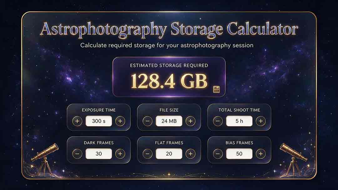
This guide explains how to estimate storage for astrophotography capture, processing, and backup without relying on misleading megapixel shortcuts. It compares measured-file, uncompressed-array, and bitrate methods; distinguishes mean, median, high-percentile, and maximum file-size statistics; and explains decimal versus binary storage units. Readers learn how FITS headers, padding, HDUs, RAW compression, calibration frames, RGB conversion, drizzle, mosaics, caches, and temporary files affect project size. Original planning tools include the Four-Bucket Storage Ledger, the Capture–Process–Protect Check, and a clearly defined storage expansion ratio. Worked examples show how to calculate peak logical data, project-relative headroom, complete-copy footprint, media count, write rate, and transfer time. The article also covers integrity verification, backup limitations, retention decisions, and troubleshooting. It is designed to help astrophotographers build realistic capacity plans for single sessions, multi-night projects, planetary video, star trails, and long-term archives.
Star Trail Exposure Calculator
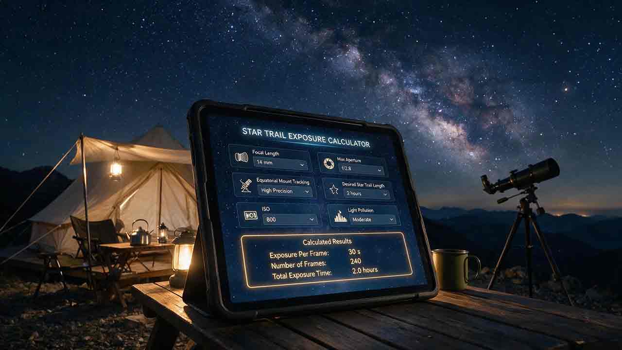
This guide explains how to calculate star-trail exposure time from Earth’s sidereal rotation, stellar declination, and local image scale. It distinguishes polar sweep, declination-adjusted sky-path length, projected pixel length, recorded sweep, missing sweep, and the full start-to-end span of a stacked sequence. Original tables compare trail lengths at several declinations, quantify one-second frame gaps at different image scales, and show how recorded time, gap time, duty cycle, and sequence sweep relate. The Trail–Frame–Sequence Check provides a practical framework for separating celestial geometry, per-frame reliability, and sequence continuity. Worked examples also address the celestial-pole edge case, local WCS-based pixel movement, frame-count limits, long-exposure noise reduction, and the difference between a single exposure and stacked frames. Readers can use the article to plan smoother trails, avoid misleading sequence calculations, and verify expected motion with native-resolution test images.
Astrophotography Image Scale Calculator
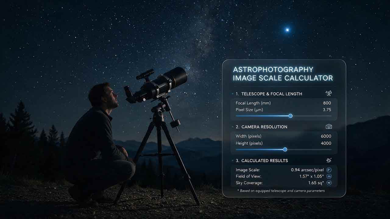
This guide explains how to calculate astrophotography image scale from camera pixel size and effective focal length, then interpret the result without confusing detector sampling with true optical resolution. It covers correct inputs, non-square pixels, reducers, amplifiers, binning, resampling, field of view, plate scale terminology, and WCS-based verification. Two original reference tables compare image scale across common pixel pitches and focal lengths and show how delivered stellar FWHM translates into pixels per FWHM. The original Scale–Quality–Target Check provides a practical decision framework for matching sampling to real image quality and target detail. Reproducible guidance explains how to measure representative FWHM from native-resolution data, diagnose discrepancies between calculated and plate-solved scale, and derive a local effective focal length. The article also distinguishes wide-field, small-target, lunar, planetary, photometric, and astrometric use cases while avoiding universal purchasing claims or unsupported equipment-testing conclusions.
Explore More Topics
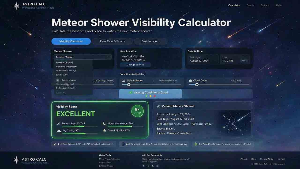
Meteor Shower Visibility Calculator
This guide explains how to use a meteor shower visibility calculator to identify a locally favorable observing window instead of relying only on a published peak time or Zenithal Hourly Rate. It covers activity periods, radiant altitude, astronomical darkness, Moon timing, weather, limiting magnitude, population index, and the distinction between named-shower members, sporadic meteors, and meteors from overlapping showers. The article introduces two original planning tools: the Five-Layer Meteor Test and the Meteor Opportunity Window, which calculates the overlap between activity, radiant, darkness, Moon, weather, and session constraints. A reproducible cross-midnight example compares illustrative 20° and 40° radiant thresholds, producing windows of 2 hours 20 minutes and 1 hour 40 minutes. Practical guidance addresses moonlight, viewing direction, dark adaptation, calculator disagreements, troubleshooting, and responsible site selection, supported by NASA, IMO, AMS, and U.S. Naval Observatory sources.
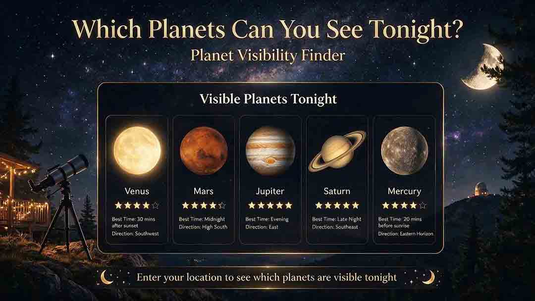
Planet Visibility Finder: Which Planets Can You See Tonight?
This guide explains how to use a planet visibility finder to decide which planets are realistically observable for a selected date, time, and location. It shows why an object being above the horizon does not guarantee visibility and explains the roles of altitude, azimuth, apparent magnitude, solar elongation, twilight, moonlight, weather, and local obstructions. Readers learn which planets are normally visible without a telescope, how Mercury and Venus differ from the outer planets, and why two finders may produce different results. The article introduces an original Four-Gate Visibility Test covering position, solar light, detectability, and site timing, plus a reproducible Useful Viewing Window calculation. A hypothetical example compares a 1-hour-26-minute naked-eye window with an 18-minute higher-altitude telescope window. Practical troubleshooting, safety guidance, and NASA, USNO, and JPL sources support the planning method.
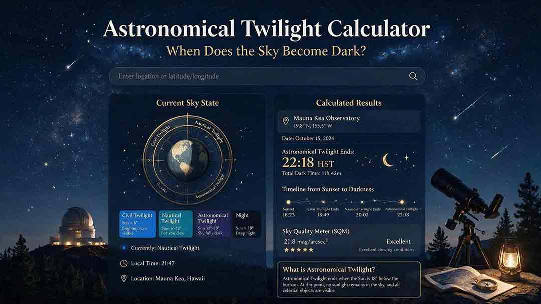
Astronomical Twilight Calculator: When Does the Sky Become Dark?
This guide explains how to use an astronomical twilight calculator to identify the end of evening astronomical twilight and the beginning of morning astronomical twilight for a selected date and location. It distinguishes sunset, civil dusk, nautical dusk, astronomical dusk, and the Sun-below-18° interval while clarifying that solar geometry does not guarantee a visibly dark sky. Readers learn how latitude, season, timezone, daylight-saving rules, moonlight, skyglow, clouds, haze, and high-latitude conditions affect practical planning. The article introduces two original tools: the Darkness Margin, which calculates how much of a session falls inside the Sun-below-18° interval, and a Task Threshold Matrix that matches observing goals to practical twilight stages. A worked cross-midnight example produces a 1-hour-48-minute dark interval. Troubleshooting guidance, planning checks, and authoritative USNO, NOAA, and National Park Service sources support the method.