Star Trail Exposure Calculator

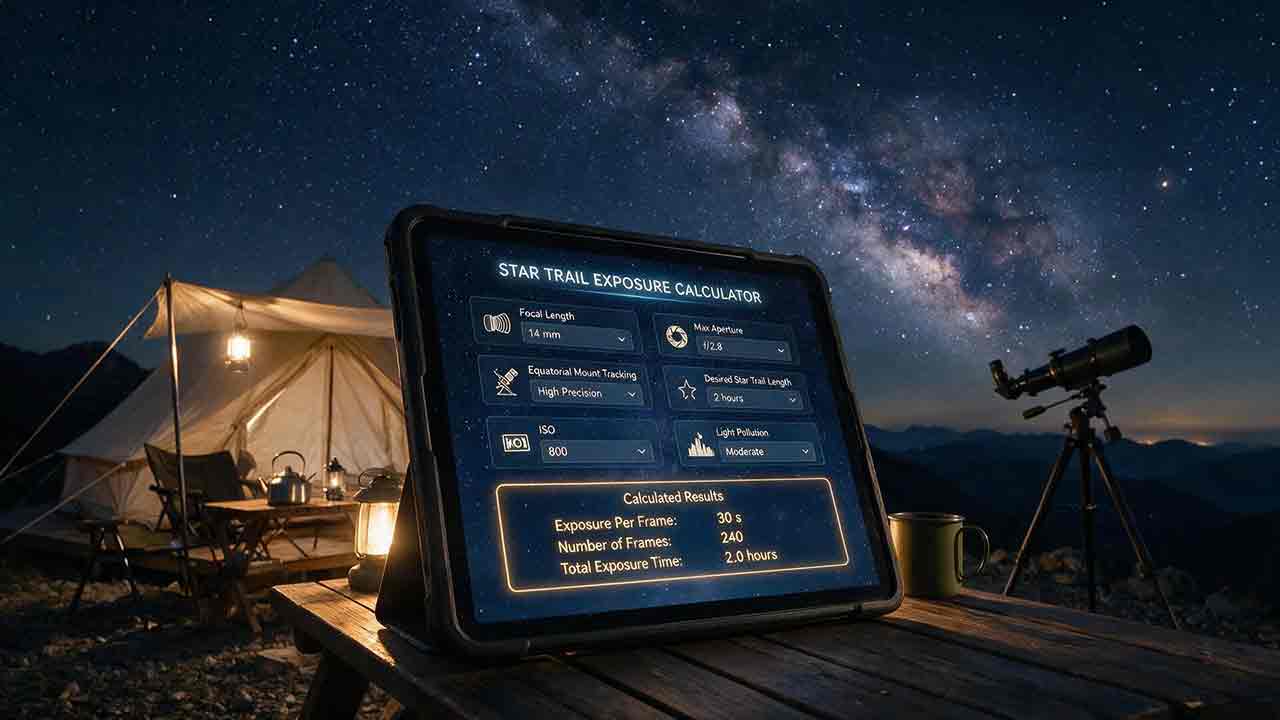
Star Trail Exposure Calculator
A Star Trail Exposure Calculator estimates how long a fixed camera must expose for a desired polar sweep, local angular trail, or pixel trail. It can also plan stacked sequences by separating recorded exposure time, frame-gap losses, and the full start-to-end rotation. Earth’s sidereal rate sets the motion; declination and local image geometry determine how that motion appears in the photograph.
Key Takeaways
- The celestial sphere rotates relative to a fixed camera by approximately 15.041069° per hour.
- The corresponding path rate at the celestial equator is approximately 15.041069 arcseconds per second.
- At declination
δ, idealized local path length is reduced by|cos δ|. - A stacked sequence has three different sweep values: recorded sweep, missing sweep, and start-to-end sweep.
- Pixel trail length should use the local image scale in the direction of motion, not blindly rely on one global center value.
This guide explains exposure-to-trail calculations, trail-to-exposure calculations, declination effects, pixel conversion, frame count, interval gaps, duty cycle, long-exposure noise reduction, and ways to verify the result with a real image.
Method note: The angular-rate constant was calculated from the JPL mean sidereal day of 86,164.09054 seconds. Angular tables, gap tables, recorded sweeps, missing sweeps, start-to-end sweeps, duty cycles, and worked examples were recalculated in a separate pass. Angular results are rounded using conventional half-up rounding. These are mathematical planning analyses rather than field tests of a particular camera, lens, intervalometer, or observing site.
How Does the Star Trail Exposure Calculator Work?
This guide separates star-trail planning into three calculation modes:
- Exposure to trail: Determine the trail produced by a known exposure.
- Trail to exposure: Determine the exposure required for a desired angular or pixel trail.
- Sequence planning: Calculate frame count, recorded time, missing time, duty cycle, and total start-to-end rotation.
The underlying celestial rate is the same in all three modes. The interpretation of the output is not.
What Is the Correct Sidereal Rotation Rate?
Earth’s mean sidereal day is:
86,164.09054 seconds
= 23 hours, 56 minutes, 4.09054 seconds
The celestial sphere’s polar rotation rate is:
360° ÷ 86,164.09054 seconds
= 0.00417807° per second
= 0.250684° per minute
= 15.041069° per hour
The equivalent path rate at the celestial equator is:
15.041069 arcseconds per second
At declination δ, the idealized small-circle path rate is:
15.041069 × |cos δ|
arcseconds per second
The JPL Astrodynamic Parameters reference lists the mean sidereal day as 86,164.09054 seconds. NASA’s Reference Systems guide explains that Earth’s rotation relative to the fixed stars is approximately 3 minutes and 56 seconds shorter than a mean solar day.
Using 15° per hour is reasonable for quick mental planning. A calculator should use the sidereal value when it displays more precise results.
For four hours:
Using 15° per hour:
4 × 15
= 60.00°

Using the mean sidereal rate:
4 × 15.041069
= 60.16°
Which Kind of Star-Trail Length Are You Calculating?
The phrase “star-trail length” can describe several different quantities.
| Measurement | Meaning | Best use |
|---|---|---|
| Polar sweep angle | Rotation around the celestial pole | Planning circular arcs and total sequence rotation |
| Sky-path length | Angular distance traveled along a star’s declination circle | Comparing stars at different declinations |
| Pixel trail length | Projected trail length on the detector | Evaluating visible motion and frame gaps |
| Endpoint separation | Straight or projected separation between start and end positions | Framing or exact endpoint placement |
These values should not be treated as interchangeable.
How Do You Calculate Polar Sweep?
Polar sweep depends only on elapsed time.
Polar sweep in degrees
= 15.041069
× exposure time in hours
Rearranged:
Exposure time in hours
= desired polar sweep in degrees
÷ 15.041069
A 15° polar sweep requires:
15 ÷ 15.041069
= 0.99727 hours
≈ 59 minutes, 50 seconds
A 30° polar sweep requires:
30 ÷ 15.041069
= 1.99454 hours
≈ 1 hour, 59 minutes, 40 seconds
Polar sweep describes rotation around the celestial pole. It does not mean that every star traces the same angular path length.
How Does Declination Change Trail Length?
A star near the celestial equator travels along a larger small circle than a star near a celestial pole.
For a representative star at declination δ:
Sky-path length in degrees
≈ polar sweep in degrees
× |cos δ|
Equivalently:
Sky-path length
≈ 15.041069
× exposure time in hours
× |cos δ|
Rearranged:
Exposure time in hours
≈ desired path length in degrees
÷ (
    15.041069
    × |cos δ|
  )
Declination is the celestial-coordinate equivalent of latitude. NASA’s celestial-coordinate guide identifies the celestial equator as 0° declination and the celestial poles as +90° and −90°.
Examples:
At 0° declination:
|cos 0°| = 1.000

At 30° declination:
|cos 30°| ≈ 0.866

At 60° declination:
|cos 60°| = 0.500

At 80° declination:
|cos 80°| ≈ 0.174
A star at 60° declination travels approximately half the path length of a star at the celestial equator during the same elapsed time.
Why Does the Cosine Factor Appear?
A declination circle is a smaller circle around the celestial axis.
For a polar sweep θ in radians, the path length on a unit celestial sphere is:
Small-circle arc length
= |cos δ| × θ
The factor |cos δ| represents the radius of the declination circle relative to the celestial equator.
This formula describes distance traveled along the arc. It does not describe the straight chord between the two endpoints.
Polar Declination Edge Case
At exactly +90° or −90° declination:
|cos δ| = 0
The idealized local sky-path length of the exact celestial pole is zero regardless of elapsed time.
A calculator should therefore handle the case explicitly:
If |cos δ| = 0
and calculating trail from exposure:

    local trail length = 0
If |cos δ| = 0
and requested trail length > 0:

    no finite exposure solution exists
A requested trail length of zero does not define one unique exposure time, because the exact pole remains at the center of rotation for any duration.
Do not round a star near the pole to exactly 90°. Use the star’s actual declination.
Very small cosine values can produce extremely long inverse-exposure estimates. Near a celestial pole, precise framing, sky brightness, weather, foreground conditions, and the star’s actual distance from the pole are often more important than additional decimal precision.
How Long Will Star Trails Be?
The following original table compares polar sweep with path length at four declinations.
Each row assumes a fixed camera and uninterrupted elapsed exposure.
| Exposure span | Polar sweep | Path at 0° Dec | Path at 30° Dec | Path at 60° Dec | Path at 80° Dec |
|---|---|---|---|---|---|
| 10 minutes | 2.51° | 2.51° | 2.17° | 1.25° | 0.44° |
| 30 minutes | 7.52° | 7.52° | 6.51° | 3.76° | 1.31° |
| 60 minutes | 15.04° | 15.04° | 13.03° | 7.52° | 2.61° |
| 120 minutes | 30.08° | 30.08° | 26.05° | 15.04° | 5.22° |
| 240 minutes | 60.16° | 60.16° | 52.10° | 30.08° | 10.45° |
The entire sky shares the same polar sweep. Local path length differs because stars trace declination circles of different radii.
Arc Length Is Not Endpoint Separation
The declination-adjusted formula calculates distance traveled along the star’s curved path.
For a small-circle path with polar sweep θ in radians:
Arc length on a unit celestial sphere
= |cos δ| × θ
The straight chord between the beginning and end is a different quantity.
For short trails, arc length and chord length can be similar. For long circular trails, they can differ substantially.
Use arc length when estimating the amount of trail recorded. Use projection-aware coordinates when exact start and end locations matter.
How Do You Calculate Pixel Trail Length?
Pixel length requires angular movement and local image geometry.
For square pixels and a locally uniform, approximately rectilinear field:
Trail length in pixels
≈ 15.041069
× exposure time in seconds
× |cos δ|
÷ local image scale along the trail
Here, local image scale along the trail means the angular distance represented by one pixel in the instantaneous direction of motion.
Rearranged:
Exposure time in seconds
≈ desired pixel trail length
× local image scale along the trail
÷ (
    15.041069
    × |cos δ|
  )
For a simple field with approximately equal horizontal and vertical scales, image scale can be estimated as:
Image scale in arcseconds per pixel
≈ 206.265
× pixel size in microns
÷ effective focal length in millimeters
Use the Astrophotography Image Scale Calculator when converting camera pixel pitch and focal length into arcseconds per pixel.
When One Image-Scale Number Is Not Enough
One scalar image scale may be inadequate when:
- horizontal and vertical pixel scales differ;
- pixels are not square;
- lens distortion is significant;
- the lens uses a fisheye projection;
- a long curved trail crosses a large part of the frame;
- the trail direction changes relative to the pixel axes;
- WCS scale varies with field position.
In those cases, calculate displacement from the local World Coordinate System rather than dividing by one center-scale value.
For a long projected trail, sample the celestial position at several times:
Total projected pixel path
≈ Σ distance(
    projected position at time i,
    projected position at time i + 1
  )
This segmented method follows the changing local direction and scale more accurately than applying one value to the complete arc.
Pixel-Length Example
Suppose:
Local image scale along the trail:
20 arcseconds per pixel

Representative declination:
30°

Desired trail length:
500 pixels
Then:
Exposure time
≈ 500 × 20
÷ (
    15.041069
    × cos 30°
  )

≈ 768 seconds
≈ 12 minutes, 48 seconds
This is a local projected estimate.
It does not mean every star in a wide or distorted frame will produce a 500-pixel trail.
What Inputs Should You Use?
A calculation may require:
- exposure time or desired trail length;
- declination of a representative star or field region;
- local image scale when a pixel result is needed;
- exposure duration per frame;
- measured end-to-start gap;
- frame count;
- available sequence duration;
- desired recorded exposure time.
Use the Correct Declination
For a narrow field, use the declination of the target region or a representative star near the center.
For a wide field, use several declinations because one value cannot describe all stars.
A useful approach is to calculate:
- the lowest declination in the important area;
- the central declination;
- the highest declination;
- the celestial-equator rate as an upper path-rate reference.
Because cosine is symmetric:
|cos(+δ)| = |cos(−δ)|
North and south declinations of equal magnitude have the same idealized path-rate factor.
Use Image Scale, Not Crop Factor
Crop factor does not change Earth’s rotation or the angular speed of the celestial sphere.
Pixel trail length depends on:
- effective focal length;
- pixel pitch;
- local image projection;
- trail direction.
Sensor dimensions affect the total frame but do not directly enter the local angular-motion formula.
Use the Camera Field of View Calculator when deciding whether a celestial pole, foreground, or intended trail pattern fits inside the frame.
Input Limits
For angular and pixel calculations:
- exposure time must be greater than zero;
- declination must be between −90° and +90°;
- image scale must be greater than zero;
- desired trail length cannot be negative;
- all units must be explicit;
- nonnumeric values are invalid.
For sequence calculations:
- per-frame exposure
Emust be greater than zero; - measured gap
Gmust be zero or greater; - scheduled frame count
Nmust be an integer of at least one; - available duration
Tmust be zero or greater; - desired recorded duration
Cmust be zero or greater; - all time values must use the same unit.
The calculator should return an explanatory message rather than Infinity, NaN, or a generic error when an inverse calculation has no finite solution.
The Trail–Frame–Sequence Check
Original framework: The Trail–Frame–Sequence Check was created for this guide to separate celestial geometry, per-frame reliability, and sequence continuity. It is an editorial planning framework rather than an industry standard or a guarantee of a particular photographic result.
Use the checks in this order:
Trail geometry
→ frame reliability
→ sequence continuity
1. Trail Geometry: What Do You Want to Record?
Choose the quantity that matches the composition:
- polar sweep angle;
- declination-adjusted sky-path length;
- projected pixel length;
- start-to-end sequence span.
A composition centered on a celestial pole is usually easiest to plan by polar sweep. A tighter non-polar composition may be easier to plan by local pixel length.
2. Frame Reliability: How Long Can Each Exposure Be?
A mathematically valid exposure can still be impractical as one frame.
Per-frame duration may be limited by:
- sky brightness;
- Moon illumination;
- foreground highlights;
- sensor heating;
- hot pixels;
- battery life;
- passing aircraft or satellites;
- tripod movement;
- wind;
- shutter or bulb-timer limits;
- risk of losing one long exposure.
Choose a per-frame duration that produces a dependable file before optimizing total trail length.
3. Sequence Continuity: What Happens Between Frames?
For stacked trails, the sky continues moving when the shutter is closed.
Possible delay sources include:
- intervalometer behavior;
- write time;
- shutter operation;
- in-camera processing;
- long-exposure noise reduction;
- timer precision;
- storage or battery interruption.
Sequence planning must distinguish the sky’s full start-to-end movement from the movement actually recorded during open-shutter periods.
How Do You Plan a Stacked Star-Trail Sequence?
Let:
E= exposure duration per frame;G= measured end-to-start gap;N= integer number of frames.
G is the measured time from the end of one exposure to the start of the next—not merely the number displayed in an interval-timer menu.
Measured gap
= next frame start time
− previous frame end time
If a camera defines an interval from one frame start to the next:
Approximate gap
= start-to-start interval
− actual exposure duration
Write time, shutter operation, post-capture processing, timer precision, and firmware behavior can make the measured value differ from that subtraction.
Recorded Sweep Versus Start-to-End Sweep
For a stacked sequence, three time quantities must be kept separate.
Recorded Exposure Time
Recorded exposure time
= N × E
Total Missing Time
Missing time
= (N − 1) × G
There is normally no internal gap after the final frame when calculating the span from the beginning of the first exposure to the end of the last.
Start-to-End Sequence Span
Total sequence span
= N × E
+ (N − 1) × G
The corresponding polar-sweep quantities are:
Recorded polar sweep
= 15.041069
× recorded exposure time in hours
Missing polar sweep
= 15.041069
× missing time in hours
Start-to-end polar sweep
= recorded polar sweep
+ missing polar sweep
The start-to-end sweep describes the angular separation between the start of the first recorded segment and the end of the last recorded segment.
The recorded sweep is the sum of the trail segments captured while the shutter was open.
The missing sweep is distributed among the internal frame gaps.
For a representative declination δ:
Recorded sky-path length
≈ recorded polar sweep
× |cos δ|
Missing sky-path length
≈ missing polar sweep
× |cos δ|
Start-to-end sky-path span
≈ start-to-end polar sweep
× |cos δ|
What Is Sequence Duty Cycle?
Duty cycle is the fraction of the full start-to-end span during which the shutter was open.
Duty cycle
= recorded exposure time
÷ total sequence span
× 100%
A high duty cycle means relatively little time was missed overall.
It does not guarantee invisible gaps. A repeated one-pixel gap can remain visible even when total missing time is small.
How Many Frames Fit in a Fixed Time Window?
For an available duration T:
Maximum complete frame count
= max(
    0,
    floor[
      (T + G)
      ÷ (E + G)
    ]
  )
The formula correctly uses N − 1 gaps.
If:
T < E
then no complete frame fits:
Maximum complete frame count = 0
Do not force the result to one frame when the available window is shorter than the required exposure.
How Many Frames Provide a Desired Recorded Time?
For desired recorded duration C:
Required frame count
= ceiling(C ÷ E)
The actual recorded duration is:
Actual recorded time
= required frame count × E
The actual value may exceed the requested duration because the final frame normally cannot be fractional.
After determining N, calculate the start-to-end span:
Total sequence span
= N × E + (N − 1) × G
Original Sequence-Planning Table
| Frames × exposure | Gap | Recorded time | Total gap time | Total sequence span | Duty cycle | Recorded sweep | Missing sweep | Start-to-end sweep |
|---|---|---|---|---|---|---|---|---|
| 30 × 60s | 1s | 30m | 29s | 30m 29s | 98.4% | 7.52° | 0.12° | 7.64° |
| 60 × 120s | 1s | 2h | 59s | 2h 00m 59s | 99.2% | 30.08° | 0.25° | 30.33° |
| 90 × 120s | 1s | 3h | 1m 29s | 3h 01m 29s | 99.2% | 45.12° | 0.37° | 45.50° |
| 120 × 180s | 2s | 6h | 3m 58s | 6h 03m 58s | 98.9% | 90.25° | 0.99° | 91.24° |
The recorded-sweep column represents trail segments captured while the shutter was open.
The start-to-end column includes the sky’s motion during all internal gaps.
How Large Is One Frame Gap?
For a gap of G seconds at declination δ:
Angular gap in arcseconds
≈ 15.041069
× G
× |cos δ|
For square pixels and a locally uniform field:
Gap in pixels
≈ angular gap
÷ local image scale along the trail
When the horizontal and vertical scales differ or the field is distorted, use the local WCS transformation in the trail direction.
One-Second Gap by Local Image Scale
| Local image scale | Gap at 0° Dec | Gap at 30° Dec | Gap at 60° Dec |
|---|---|---|---|
| 10″/pixel | 1.50 px | 1.30 px | 0.75 px |
| 20″/pixel | 0.75 px | 0.65 px | 0.38 px |
| 40″/pixel | 0.38 px | 0.33 px | 0.19 px |
| 80″/pixel | 0.19 px | 0.16 px | 0.09 px |
A subpixel result does not guarantee that a gap will be invisible.
Visibility also depends on:
- star brightness;
- point-spread-function width;
- contrast;
- output enlargement;
- sharpening;
- compositing method;
- local distortion;
- trail direction.
No photons are recorded during the gap, regardless of whether processing makes the break difficult to see.
Total Missing Path Is Not One Continuous Break
Total missing path is the sum of all internal gaps.
Total missing angular path
= one-gap angular path
× number of gaps
For 90 frames there are normally 89 internal gaps.
The total does not represent one continuous 89-second break unless the sequence actually stopped for that duration.
For visual continuity, evaluate both:
- the size of each individual gap;
- the number and regularity of repeated gaps.
A sequence with many small gaps can produce a dotted or segmented appearance even when the overall duty cycle is high.
Sequence Example: 90 Two-Minute Frames
Suppose:
Frames:
90

Exposure per frame:
120 seconds

Measured end-to-start gap:
1 second
Recorded exposure time:
90 × 120
= 10,800 seconds
= 3 hours
Total missing time:
89 × 1
= 89 seconds
= 1 minute, 29 seconds
Start-to-end span:
10,800 + 89
= 10,889 seconds
= 3 hours, 1 minute, 29 seconds
Recorded polar sweep:
15.041069 × 3
= 45.12°
Missing polar sweep:
15.041069 × 89 ÷ 3,600
= 0.37°
Start-to-end polar sweep:
45.12° + 0.37°
= 45.50°
The final trail extends from an initial point to an endpoint separated by approximately 45.50° of polar rotation.
The camera recorded approximately 45.12° of trail segments. Approximately 0.37° was distributed among 89 unrecorded intervals.
At 30° declination, each one-second gap represents:
15.041069 × cos 30°
= 13.03 arcseconds
At a local scale of 20 arcseconds per pixel:
13.03 ÷ 20
= 0.65 pixel
This predicts relatively small individual gaps, but a test sequence is still necessary because repeated boundaries, processing, contrast, and local projection affect visibility.
Single Long Exposure or Stacked Frames: Which Is Better?
Neither method is universally better.
| Consideration | Single long exposure | Stacked sequence |
|---|---|---|
| Trail continuity | Continuous while the shutter is open | Depends on measured gaps |
| File count | One main sky frame | Many frames |
| Failure risk | One failure can ruin the full sky exposure | Damaged frames may be removable |
| Sky brightness | Can become difficult to control | Easier to manage per frame |
| Foreground exposure | Tied to the same exposure unless composited | Can be planned separately |
| Sensor heat | Sustained through one long exposure | Still accumulates, but capture is segmented |
| Processing | Simpler file management | Requires sequence compositing |
| Aircraft or satellite contamination | May affect the full exposure | Individual frames may be repairable |
| Gap risk | None during the exposure | Requires timer and processing control |
| Final trail duration | Fixed at capture | Can often be shortened during processing |
When a Single Exposure Makes Sense
A single long exposure can be practical when:
- the sky remains within usable brightness limits;
- the camera supports the required bulb or time exposure;
- uninterrupted trails are the priority;
- battery and storage are reliable;
- losing one file is an acceptable risk;
- foreground movement is manageable.
Canon’s bulb-exposure documentation recommends stable support and remote or timer-based operation for long exposures and notes that long bulb exposures can produce more noise than ordinary exposures.
When a Stacked Sequence Makes Sense
Stacking can be practical when:
- one long exposure would overbrighten the sky;
- damaged frames may need to be removed;
- the final trail duration may need adjustment;
- the foreground requires a separate exposure;
- the camera cannot perform one continuous exposure;
- a testable, recoverable workflow is preferred.
A Nikon-hosted D780 star-trail example used 180-second exposures and a 181-second interval, creating an intended delay of approximately one second.
That is one documented camera workflow, not a universal interval definition.
Why Does Long-Exposure Noise Reduction Cause Gaps?
Some cameras perform a second processing or dark-frame stage after a long exposure when long-exposure noise reduction is enabled.
Canon’s EOS R5 documentation states that noise-reduction processing may take as long as the original exposure and that another picture cannot be taken until processing finishes.
Nikon’s Long Exposure NR documentation states that processing can roughly double the total recording time and prevents additional capture while processing is underway.
For a 120-second trail exposure, a processing delay of comparable duration would create a major missing segment rather than a minor frame boundary.
Before beginning a sequence:
- confirm whether long-exposure noise reduction is enabled;
- test whether the camera pauses after each frame;
- measure the actual end-to-start gap;
- decide how calibration and noise processing will be handled;
- do not assume continuous mode overrides post-capture processing.
The appropriate workflow depends on the camera, temperature, file type, and processing method. There is no universal setting for every camera.
How Should You Choose Per-Frame Exposure?
Total elapsed duration controls the overall start-to-end sweep. Per-frame duration controls file reliability and the number of frame boundaries.
Begin with the longest frame that remains dependable under the actual sky and foreground conditions—not simply the longest exposure the camera can technically record.
Shorter Frames
Potential advantages:
- less time lost when one frame fails;
- easier highlight control;
- easier removal of contaminated frames;
- more flexibility in final trail length;
- less dependence on one file.
Tradeoffs:
- more files;
- more frame boundaries;
- more chances for interval gaps;
- more shutter cycles on mechanical systems;
- greater processing workload.
Longer Frames
Potential advantages:
- fewer boundaries;
- fewer gaps;
- simpler file management;
- longer uninterrupted trail segments.
Tradeoffs:
- greater loss if one frame fails;
- increased clipping risk;
- greater thermal or hot-pixel visibility in some conditions;
- longer processing delays if noise reduction activates;
- less flexibility after capture.
Per-frame duration is primarily a reliability decision. It does not change the underlying sidereal rate.
How Does Composition Change the Calculation?
Pole-Centered Circular Trails
For a composition centered near a celestial pole, plan primarily by polar sweep.
A two-hour uninterrupted span produces approximately:
30.08° of polar sweep
Stars at different distances from the pole trace arcs of different physical lengths while sharing the same rotation angle.
Trails Near the Celestial Equator
Stars close to 0° declination have the greatest idealized sky-path rate.
This can produce long trails in less time, but their projected direction and shape depend on camera orientation and lens projection.
Wide-Angle Frames
A wide frame may contain stars across a broad range of declinations.
One declination and one image scale cannot describe the full image. Calculate several representative positions or use WCS-based prediction.
Fisheye Images
Fisheye lenses do not follow ideal rectilinear projection.
The sidereal sweep remains valid, but conversion to pixel path requires a projection-specific model or calibrated image transformation.
Does Atmospheric Refraction Affect the Result?
The sidereal and declination formulas describe ideal celestial geometry.
They do not model atmospheric refraction, which changes apparent stellar positions most strongly near the horizon.
For ordinary composition and duration planning, the effect is often secondary. For precise low-altitude endpoint prediction or WCS comparison, use observed coordinates or a model that includes:
- observing time;
- location;
- altitude;
- atmospheric pressure;
- temperature;
- wavelength or passband.
The ideal formula should not be treated as a complete physical model of low-altitude apparent motion.
How Can You Verify the Real Trail Geometry?
Capture a short native-resolution sequence, plate-solve a frame, and compare predicted movement with measured movement.
Astropy’s World Coordinate System documentation describes transformations between image pixels and celestial coordinates.
A robust verification can:
- identify representative stars and their declinations;
- calculate or inspect local directional image scale;
- compare movement at several field positions;
- inspect distortion near the edges;
- measure actual end-to-start frame gaps;
- confirm that the image has not been resized or cropped;
- compare predicted and recorded trail segments.
For long trails, transform sampled celestial positions into image coordinates rather than assuming one center-scale value applies to the entire path.
Step-by-Step Star-Trail Workflow
Step 1: Choose the Composition
Decide whether the photograph is based on:
- circles around a celestial pole;
- diagonal arcs;
- near-horizontal streaks;
- a landscape foreground;
- a wide or fisheye projection.
Step 2: Select the Trail Quantity
Use:
- polar sweep for pole-centered arcs;
- declination-adjusted path for a representative star;
- local pixel length for close detector-level planning.
Step 3: Check the Field of View
Confirm that the celestial pole, foreground, and expected trails remain inside the usable frame.
Step 4: Choose a Reliable Per-Frame Exposure
Balance continuity against sky brightness, clipping, battery use, and failure risk.
Step 5: Measure the Real Gap
Run several frames and measure:
next frame start
− previous frame end
Do not rely only on the interval displayed in the camera menu.
Step 6: Check Camera Processing
Verify:
- long-exposure noise reduction;
- write time;
- buffer behavior;
- bulb or time mode;
- interval semantics;
- maximum programmable exposure;
- storage;
- external power.
Step 7: Calculate Sequence Quantities
Calculate:
- recorded time;
- total missing time;
- start-to-end span;
- duty cycle;
- recorded sweep;
- missing sweep;
- start-to-end sweep.
Step 8: Capture a Short Test Sequence
Inspect:
- trail brightness;
- highlight clipping;
- focus;
- individual gap visibility;
- repeated gap pattern;
- tripod stability;
- foreground exposure;
- condensation or dew.
Step 9: Record the Plan
Record:
- center coordinates;
- camera orientation;
- representative declination;
- local image scale;
- frame exposure;
- measured gap;
- frame count;
- total duration;
- expected sweep;
- battery and storage requirements.
Common Star-Trail Calculation Mistakes
Using a 24-Hour Solar Day
Star-trail calculations should use the sidereal day because movement is measured relative to the stars.
Treating 15.041069 Arcseconds per Second as Every Star’s Path Rate
That value is the path rate at the celestial equator. Multiply by |cos δ| for another declination.
Confusing Recorded Sweep with Start-to-End Sweep
The sky moves during frame gaps, but the camera does not record those missing segments.
Applying Crop Factor to the Sidereal Rate
Crop factor does not alter celestial motion. Use local image scale when converting angular movement into pixels.
Ignoring Declination
One hour does not produce the same path length at 0° and 80° declination.
Dividing by Zero at the Celestial Pole
An inverse positive-length calculation has no finite solution at exactly ±90° declination.
Confusing Arc Length with Endpoint Separation
Long trails are curved. Distance traveled along the arc is not the same as the chord between endpoints.
Adding a Gap After the Final Frame
A sequence of N frames normally contains N − 1 internal gaps.
Assuming the Interval Setting Equals the Gap
Some cameras use start-to-start intervals. Others apply a delay after the exposure. Measure the real end-to-start time.
Treating Total Missing Path as One Large Break
Many small gaps are distributed throughout the trail. They do not form one continuous break unless the sequence actually stops.
Leaving Long-Exposure Noise Reduction Unchecked
Post-capture processing can create delays comparable to the exposure itself on some cameras.
Using One Center Image Scale Across a Distorted Frame
Pixel movement can vary with field position and trail direction.
Troubleshooting
| Problem | Possible cause | Practical response |
|---|---|---|
| Trails contain regular dotted gaps | End-to-start delay, write time, processing, or long-exposure noise reduction | Measure the actual gap and inspect camera processing settings |
| Duty cycle is high but gaps remain visible | Individual gaps are repeated and large relative to the local PSF | Evaluate per-gap pixels, not only total missing time |
| Start-to-end sweep exceeds recorded trail length | The sequence includes unrecorded internal gaps | Compare recorded, missing, and start-to-end sweeps separately |
| Gap size changes across the frame | Declination, distortion, or directional image scale varies | Use local WCS measurements at several positions |
| Trails are shorter than expected | Declination, recorded time, or unit conversion is wrong | Recalculate with the correct cosine and exposure duration |
| Trails are longer than expected | Start-to-end span was mistaken for recorded time or units were mixed | Separate open-shutter time from total elapsed time |
| Calculator returns infinity near the pole | The inverse formula divided by a near-zero cosine | Use the exact polar edge-case logic and actual declination |
| Circular trails are off-center | The celestial pole is outside the intended frame location | Reframe with a sky-planning or plate-solving tool |
| Sky becomes too bright before the desired sweep is reached | Per-frame exposure is too long for the conditions | Use shorter stacked frames or change capture conditions |
| Foreground is blurred or clipped | The sky and foreground require different exposures | Capture and disclose a separate foreground frame when appropriate |
| One failed frame creates a large break | Per-frame exposure is too long | Shorten individual frames or plan a repairable workflow |
| Sequence stops early | Battery, storage, thermal, timer, or buffer limitation | Test the complete capture chain in advance |
| Pixel prediction disagrees with the image | Local scale, distortion, resize, crop, or focal length is wrong | Verify native image geometry and WCS |
| Trails show vibration rather than smooth celestial movement | Wind, shutter operation, tripod motion, or unstable ground | Stabilize the setup and use remote or timed release |
Practical Recommendations by Use Case
For Smooth Trails with Processing Flexibility
Use a stacked sequence with the smallest reliable measured gap.
Calculate individual gap size, total missing time, recorded sweep, and start-to-end sweep.
For Minimal Processing
Use a single long exposure only when sky brightness, foreground, power, and camera operation make it dependable.
Run a shorter test first because one interruption can affect the complete exposure.
For Pole-Centered Circles
Plan with:
Exposure hours
= desired sweep degrees
÷ 15.041069
Use field-of-view planning to place the pole deliberately.
For Non-Polar Trails
Use the representative star’s actual declination.
Do not assume that the celestial-equator path rate applies throughout the frame.
For Pixel-Level Planning
Use local image scale along the trail.
For a wide or distorted field, sample projected positions through the WCS instead of applying one global value.
For a Separate Foreground
Capture the sky and foreground according to their different exposure needs.
When publishing the image, describe it accurately as a composite when separate frames were combined.
Field Checklist
Before starting:
- Confirm that the camera is fixed rather than tracking.
- Confirm center coordinates and orientation.
- Identify representative declinations.
- Choose polar sweep, sky-path length, or pixel trail as the planning quantity.
- Calculate local image scale when pixel length matters.
- Handle exact or near-polar declinations correctly.
- Select a reliable per-frame exposure.
- Measure the true end-to-start gap.
- Check long-exposure noise reduction.
- Confirm bulb, time, and interval behavior.
- Calculate frame count.
- Calculate recorded time and total gap time.
- Calculate recorded, missing, and start-to-end sweep.
- Confirm battery and storage capacity.
- Stabilize the tripod.
- Focus using a bright star.
- Capture a short test sequence.
- Inspect clipping, focus, gaps, repetition, and foreground movement.
- Record the final settings.
Use the Moon Phase Calculator to evaluate lunar illumination and the Rule of 500 Calculator for Milky Way Photography when the goal changes from deliberate trails to shorter untracked stars.
Site Access and Night-Shooting Safety
A favorable calculation does not establish that a location is open, safe, or legally accessible.
Before setting up:
- follow property rules and posted hours;
- obtain permits when required;
- do not enter private land without permission;
- avoid blocking roads, trails, gates, and emergency access;
- follow fire, wildlife, weather, and nighttime-use restrictions;
- secure equipment against wind and unstable ground;
- avoid lighting that creates a hazard for other visitors;
- do not leave equipment unattended where prohibited or unsafe.
This article provides photographic planning information, not legal or site-access advice.
Practical Conclusion
The Star Trail Exposure Calculator separates three quantities that are often confused:
Recorded trail
Missing trail
Start-to-end trail span
Use the sidereal rate for polar rotation:
Polar sweep
= 15.041069°
× elapsed hours
Use declination for local path length:
Sky path
≈ polar sweep
× |cos declination|
Use local directional image scale or a WCS transformation when pixel accuracy matters.
Choose the trail geometry
→ validate each frame
→ measure the gaps
→ separate recorded and missing motion
For pole-centered circles, plan by sweep angle. For non-polar trails, include declination. For stacked sequences, never treat the full start-to-end rotation as though every part of it was recorded.
Frequently Asked Questions
How Long Does a 30° Star Trail Take?
A 30° polar sweep takes approximately 1 hour, 59 minutes, and 40 seconds at the mean sidereal rate. The path traveled by a particular star is shorter away from the celestial equator.
Does Focal Length Change How Fast Stars Move?
No. Earth’s rotation and stellar declination determine angular motion. Focal length changes how large that angular movement appears on the detector.
Does Crop Factor Affect Star-Trail Exposure Time?
No. Crop factor does not change sidereal rotation. Sensor dimensions change framing, while focal length, pixel pitch, and local projection affect trail length in pixels.
Why Is Start-to-End Sweep Longer Than Recorded Sweep?
The sky continues rotating during frame gaps. Start-to-end sweep includes that missing motion, while recorded sweep includes only open-shutter periods.
What Happens at Exactly 90° Declination?
The exact celestial pole has zero idealized local path radius. A forward calculation returns zero local trail length, and a request for a positive path length has no finite exposure solution.
Why Are There Gaps in Stacked Star Trails?
The shutter is closed between frames. Common causes include timer delay, write time, shutter operation, post-capture processing, and long-exposure noise reduction.
Sources
NASA Jet Propulsion Laboratory — Astrodynamic Parameters
Mean sidereal-day duration and related astronomical constants. Accessed August 1, 2026.NASA Science — Basics of Space Flight: Reference Systems
Earth’s rotation relative to the Sun and fixed stars. Accessed August 1, 2026.NASA Science — The Celestial Sphere, Declination, and Right Ascension
Declination, right ascension, the celestial equator, and the celestial poles. Accessed August 1, 2026.NASA Science — Universe Glossary
Definitions of declination, angular units, equatorial coordinates, and exposure. Accessed August 1, 2026.Nikon USA — Star Trails with the Nikon D780
Manufacturer-hosted example using 180-second exposures and a 181-second interval. Accessed August 1, 2026.Nikon — Long Exposure Noise Reduction
Official explanation of post-exposure noise-reduction processing and its effect on recording time. Accessed August 1, 2026.Canon — Long Exposure Noise Reduction
Official documentation on long-exposure noise-reduction processing and camera availability. Accessed August 1, 2026.Canon — Bulb Exposures and Bulb Timer
Official guidance on bulb exposure, remote operation, tripods, and long-exposure noise. Accessed August 1, 2026.Astropy — World Coordinate System
Pixel-to-celestial-coordinate transformations for checking image geometry and local projected trail movement. Accessed August 1, 2026.OpenStax Astronomy 2e — Earth and Sky
Celestial coordinates, apparent sky rotation, right ascension, and declination. Accessed August 1, 2026.
More from Astrophotography Planning Tools
Astrophotography Storage Calculator
This guide explains how to estimate storage for astrophotography capture, processing, and backup without relying on misleading megapixel shortcuts. It compares measured-file, uncompressed-array, and bitrate methods; distinguishes mean, median, high-percentile, and maximum file-size statistics; and explains decimal versus binary storage units. Readers learn how FITS headers, padding, HDUs, RAW compression, calibration frames, RGB conversion, drizzle, mosaics, caches, and temporary files affect project size. Original planning tools include the Four-Bucket Storage Ledger, the Capture–Process–Protect Check, and a clearly defined storage expansion ratio. Worked examples show how to calculate peak logical data, project-relative headroom, complete-copy footprint, media count, write rate, and transfer time. The article also covers integrity verification, backup limitations, retention decisions, and troubleshooting. It is designed to help astrophotographers build realistic capacity plans for single sessions, multi-night projects, planetary video, star trails, and long-term archives.
Camera Field of View Calculator
This guide explains how to calculate horizontal, vertical, and diagonal camera field of view from the recorded active sensor dimensions and effective focal length. It distinguishes physical focal length from crop-factor comparisons, shows why aspect ratio and target rotation affect framing, and provides independently calculated reference tables for common sensor sizes and focal lengths. The original Frame Envelope Check separates ideal frame geometry, the target envelope, and the usable frame retained after dithering, registration, distortion correction, and cropping. Worked examples demonstrate target occupancy, maximum permitted focal length, rotated bounding boxes, and mosaic panel counts with overlap. The article also explains radians versus degrees, crop and stabilization modes, focus breathing, rectilinear versus fisheye projection, and plate-solving verification through a celestial WCS. Readers can use the formulas, margin budget, troubleshooting table, and framing checklist to plan wide-field compositions, small-target imaging, or mosaics without treating a mathematical edge-to-edge fit as a guaranteed final frame.
Astrophotography Image Scale Calculator
This guide explains how to calculate astrophotography image scale from camera pixel size and effective focal length, then interpret the result without confusing detector sampling with true optical resolution. It covers correct inputs, non-square pixels, reducers, amplifiers, binning, resampling, field of view, plate scale terminology, and WCS-based verification. Two original reference tables compare image scale across common pixel pitches and focal lengths and show how delivered stellar FWHM translates into pixels per FWHM. The original Scale–Quality–Target Check provides a practical decision framework for matching sampling to real image quality and target detail. Reproducible guidance explains how to measure representative FWHM from native-resolution data, diagnose discrepancies between calculated and plate-solved scale, and derive a local effective focal length. The article also distinguishes wide-field, small-target, lunar, planetary, photometric, and astrometric use cases while avoiding universal purchasing claims or unsupported equipment-testing conclusions.
Explore More Topics
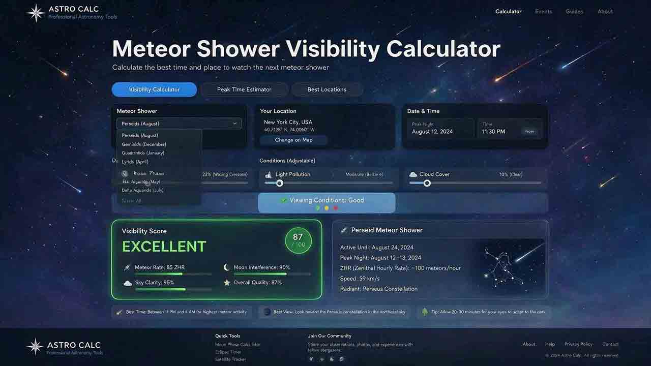
Meteor Shower Visibility Calculator
This guide explains how to use a meteor shower visibility calculator to identify a locally favorable observing window instead of relying only on a published peak time or Zenithal Hourly Rate. It covers activity periods, radiant altitude, astronomical darkness, Moon timing, weather, limiting magnitude, population index, and the distinction between named-shower members, sporadic meteors, and meteors from overlapping showers. The article introduces two original planning tools: the Five-Layer Meteor Test and the Meteor Opportunity Window, which calculates the overlap between activity, radiant, darkness, Moon, weather, and session constraints. A reproducible cross-midnight example compares illustrative 20° and 40° radiant thresholds, producing windows of 2 hours 20 minutes and 1 hour 40 minutes. Practical guidance addresses moonlight, viewing direction, dark adaptation, calculator disagreements, troubleshooting, and responsible site selection, supported by NASA, IMO, AMS, and U.S. Naval Observatory sources.
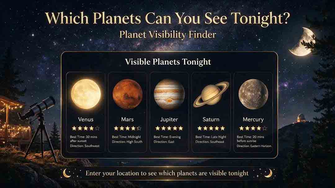
Planet Visibility Finder: Which Planets Can You See Tonight?
This guide explains how to use a planet visibility finder to decide which planets are realistically observable for a selected date, time, and location. It shows why an object being above the horizon does not guarantee visibility and explains the roles of altitude, azimuth, apparent magnitude, solar elongation, twilight, moonlight, weather, and local obstructions. Readers learn which planets are normally visible without a telescope, how Mercury and Venus differ from the outer planets, and why two finders may produce different results. The article introduces an original Four-Gate Visibility Test covering position, solar light, detectability, and site timing, plus a reproducible Useful Viewing Window calculation. A hypothetical example compares a 1-hour-26-minute naked-eye window with an 18-minute higher-altitude telescope window. Practical troubleshooting, safety guidance, and NASA, USNO, and JPL sources support the planning method.
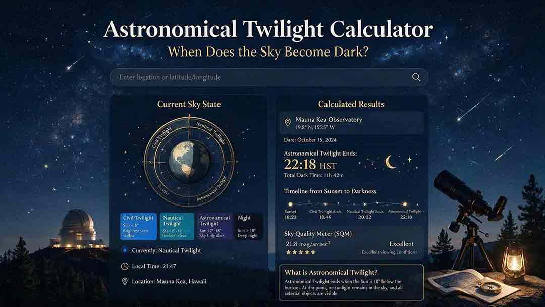
Astronomical Twilight Calculator: When Does the Sky Become Dark?
This guide explains how to use an astronomical twilight calculator to identify the end of evening astronomical twilight and the beginning of morning astronomical twilight for a selected date and location. It distinguishes sunset, civil dusk, nautical dusk, astronomical dusk, and the Sun-below-18° interval while clarifying that solar geometry does not guarantee a visibly dark sky. Readers learn how latitude, season, timezone, daylight-saving rules, moonlight, skyglow, clouds, haze, and high-latitude conditions affect practical planning. The article introduces two original tools: the Darkness Margin, which calculates how much of a session falls inside the Sun-below-18° interval, and a Task Threshold Matrix that matches observing goals to practical twilight stages. A worked cross-midnight example produces a 1-hour-48-minute dark interval. Troubleshooting guidance, planning checks, and authoritative USNO, NOAA, and National Park Service sources support the method.