Astrophotography Storage Calculator

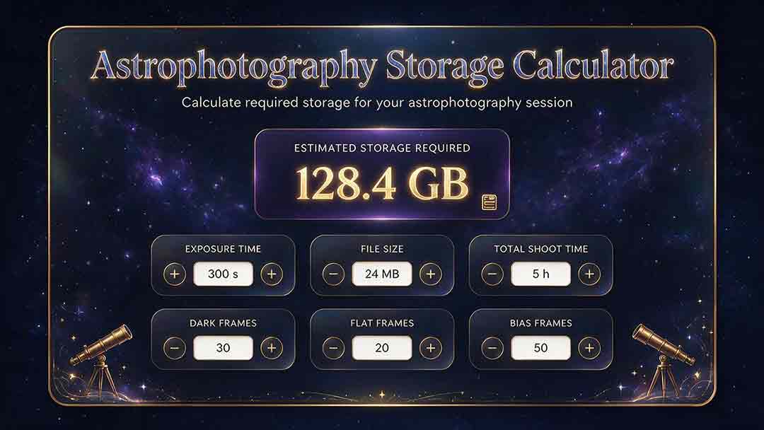
Astrophotography Storage Calculator
An Astrophotography Storage Calculator estimates how much capacity an imaging session will consume during capture, processing, and backup. For existing equipment, multiply the mean size of representative files by the planned frame count. For uncompressed data, calculate payload from image dimensions, channels, and stored bit depth, then add format overhead, processing expansion, planning headroom, and complete protected copies.
Key Takeaways
- Use the arithmetic mean of representative files to estimate expected aggregate storage.
- Keep the median, a high-percentile value, and the largest sample for different planning decisions.
- Calculate capture data, processing workspace, planning headroom, and protected copies separately.
- Distinguish decimal
GBandTBfrom binaryGiBandTiB. - FITS size depends on padded headers, padded data units, extensions, and possibly compression—not only image dimensions.
- A calculated write rate is an arithmetic minimum, not proof that a card or drive is camera-compatible.
This guide explains how to estimate RAW, FITS, video, calibration, processing, mosaic, backup, write-speed, transfer-time, and multi-night storage without treating megapixels or advertised drive capacity as complete answers.
Method note: Numerical tables and worked examples were generated from the formulas shown in this guide and checked in a separate calculation pass. Binary file values use MiB and GiB; manufacturer storage capacities commonly use decimal GB and TB. The calculations are planning analyses rather than hands-on tests of particular cameras, storage cards, drives, capture programs, or processing applications.
How Does the Astrophotography Storage Calculator Work?
Three calculation methods cover most astrophotography workflows.
| Method | Best use | Core calculation |
|---|---|---|
| Measured-file method | Camera RAW, compressed FITS, proprietary files | Representative mean file size × planned count |
| Array method | Uncompressed FITS or known image arrays | Width × height × channels × stored bits ÷ 8 |
| Bitrate method | Planetary video or continuous recording | Bitrate × duration ÷ 8 |
The calculator’s direct estimate should use only the inputs actually entered. The additional formulas in this guide extend that result to processing workspace, headroom, backup copies, transfer time, and multi-volume capture planning.
Which File-Size Statistic Should You Use?
Use the mean for expected aggregate capacity, the median for a typical individual file, and a high-percentile or conservative value when running close to a card or drive limit.
Measured-File Method
For variable-size formats, capture a representative sample using the intended:
- resolution;
- crop or region of interest;
- bit depth;
- compression;
- file format;
- camera mode;
- binning;
- scene type.
Record each file size in bytes.
Calculate the arithmetic mean:
Mean sample file size
= total logical bytes in the sample
÷ sample file count
Then estimate expected storage:
Expected storage
= mean sample file size
× planned file count
Also record:
- median file size: a useful description of a typical individual file;
- 90th or 95th percentile: a conservative value for session planning;
- largest representative file: useful for stress testing.
Why the Mean Is Better for Aggregate Storage
The total size of a collection is the sum of its files. When a representative sample reflects the intended capture conditions, its arithmetic mean directly estimates the expected bytes per future file.
A median can understate aggregate storage when a minority of files are substantially larger than the rest. It remains valuable for describing a typical file because it is less sensitive to isolated extremes.
Which Statistic Fits Which Decision?
| Statistic | Appropriate use | Main limitation |
|---|---|---|
| Mean observed file size | Expected aggregate storage | Sensitive to unrepresentative large or small samples |
| Median observed file size | Typical individual file | May underestimate total bytes in a skewed distribution |
| High-percentile file size | Conservative session or card planning | Requires a sufficiently large sample |
| Largest representative file | Capacity stress test | May overestimate ordinary storage |
| Manufacturer estimate | Initial comparison | May use different scenes, settings, firmware, or rounding |
For a card that will remain comfortably below capacity, the sample mean plus documented headroom may be sufficient. For a card expected to approach its limit, use a high-percentile or deliberately conservative file size.
How Do You Estimate an Uncompressed Image?
For a rectangular uncompressed image array:
Payload bytes
= image width
× image height
× channel count
× stored bits per sample
÷ 8
For a monochrome 6,000 × 4,000 image stored in a 16-bit container:
6,000 × 4,000 × 1 × 16 ÷ 8
= 48,000,000 bytes
That is:
48.0 MB
or approximately 45.8 MiB
This formula calculates array payload. It does not include:
- file headers;
- previews;
- metadata;
- file-format padding;
- file-system allocation;
- overscan;
- additional HDUs;
- compression;
- software-specific data structures.
How Does Bit Depth Affect Storage?
Theoretical uncompressed payload grows in direct proportion to the stored bits per sample.
16-bit data use twice the payload of 8-bit data.

32-bit data use twice the payload of 16-bit data.
The camera’s analog-to-digital converter depth does not always equal the physical number of bits allocated to each saved sample.
Possible implementations include:
- tightly packed 12-bit values;
- compressed 12-bit or 14-bit values;
- camera samples placed in a 16-bit container;
- processing data converted to 32-bit floating point;
- RGB working files containing three complete channels.
Nikon’s official NEF RAW documentation lists 12-bit and 14-bit recording together with lossless-compressed, compressed, and uncompressed modes. Its memory-card capacity table also notes that reported file sizes are approximate and can vary with the recorded scene.
Theoretical Single-Frame Payload
The following original table shows mathematical array payload before headers, padding, previews, or compression.
The packed 12-bit column is not a FITS BITPIX=12 calculation. Standard FITS image arrays do not use BITPIX=12.
| Pixel count | Tightly packed 12-bit | 16-bit container | 32-bit float | 100 frames at 16-bit |
|---|---|---|---|---|
| 6 MP | 8.6 MiB | 11.4 MiB | 22.9 MiB | 1.12 GiB |
| 12 MP | 17.2 MiB | 22.9 MiB | 45.8 MiB | 2.24 GiB |
| 24 MP | 34.3 MiB | 45.8 MiB | 91.6 MiB | 4.47 GiB |
| 36 MP | 51.5 MiB | 68.7 MiB | 137.3 MiB | 6.71 GiB |
| 60 MP | 85.8 MiB | 114.4 MiB | 228.9 MiB | 11.18 GiB |
The table does not predict the RAW size of a particular camera. Proprietary compression, previews, metadata, and storage layout can produce materially different files.
What Is the Difference Between MB, MiB, GB, and GiB?
Decimal and binary units use different divisors.
The National Institute of Standards and Technology defines:
1 MB  = 1,000,000 bytes
1 MiB = 1,048,576 bytes

1 GB  = 1,000,000,000 bytes
1 GiB = 1,073,741,824 bytes

1 TB  = 1,000,000,000,000 bytes
1 TiB = 1,099,511,627,776 bytes
A drive sold as:
1 TB
contains approximately:
931.3 GiB
before formatting, system partitions, reserved areas, or existing files are considered.
Neither value is incorrect when its unit is stated accurately. Confusion occurs when decimal and binary quantities are mixed without labeling them.
Recommended Calculator Output
A trustworthy calculator should show:
- exact bytes;
- decimal MB, GB, or TB;
- binary MiB, GiB, or TiB;
- the conversion basis used.
What Is Logical File Size Versus Space Used on Disk?
A file can have two relevant sizes.
- Logical file size: the number of bytes contained in the file.
- Allocated size: the physical space reserved for it by the file system.
File systems allocate storage in whole blocks or allocation units. A file that uses only part of its final unit still occupies the complete unit.
Therefore:
Space used on disk
may exceed
the sum of logical file bytes
The difference is usually small for large RAW or FITS frames. It can become more noticeable when a project contains many small files such as:
- logs;
- previews;
- thumbnails;
- database entries;
- sidecar files;
- scripts;
- masks;
- temporary records.
Use logical bytes for image-format calculations. Use measured allocated usage when planning the capacity of the actual volume.
How Do You Calculate a FITS File Size?
FITS stores information in Header/Data Units, or HDUs. Each header and each data section is padded separately to a multiple of 2,880 bytes.
NASA’s FITS Primer explains that every header record occupies 80 characters and that headers and data units are stored in 2,880-byte blocks.
FITS Header Size
Count every header card through and including the END card.
Unpadded header bytes
= header card count × 80
Then pad the header:
Padded header bytes
= 2,880
× ceiling(
    unpadded header bytes
    ÷ 2,880
  )
For example, a header containing 40 cards has:
40 × 80
= 3,200 unpadded bytes
It therefore occupies:
2 × 2,880
= 5,760 padded bytes
Ordinary Image-HDU Data Size
For an uncompressed primary image or ordinary image extension:
Unpadded image bytes
= |BITPIX| ÷ 8
× NAXIS1
× NAXIS2
× additional axis lengths
For a two-dimensional image:
Unpadded image bytes
= |BITPIX| ÷ 8
× NAXIS1
× NAXIS2
Then pad the data:
Padded data bytes
= 2,880
× ceiling(
    unpadded image bytes
    ÷ 2,880
  )
Generalized Extension-HDU Data Size
For a generalized uncompressed extension containing PCOUNT and GCOUNT, the NASA FITS extension rules define the unpadded data size as:
Unpadded HDU data bytes
= |BITPIX| ÷ 8
× GCOUNT
× (
    PCOUNT
    + product of all NAXISn values
  )
For an ordinary image extension:
GCOUNT = 1
PCOUNT = 0
The expression then reduces to the standard image-array calculation.
PCOUNT has extension-specific meaning. In a binary table it can include supplementary data such as a heap used by variable-length arrays. It should not be interpreted as an image dimension.
Total HDU and File Size
For one HDU:
HDU bytes
= padded header bytes
+ padded data bytes
For a multi-HDU FITS file:
FITS file bytes
= sum of all padded HDU sizes
Compressed FITS Files
Compressed-image FITS files may use specialized extensions or binary-table structures. Their physical size depends on the stored compressed content and associated HDUs.
Do not estimate a compressed FITS file solely from:
width × height × uncompressed BITPIX
Measure representative compressed files or inspect the actual HDU structure.
FITS Calculation Limits
The basic formula may not describe every file exactly when it includes:
- compressed-image extensions;
- binary tables;
- variable-length arrays;
- heaps;
- multiple image planes;
- masks;
- checksums;
- overscan;
- thumbnails;
- application-specific extensions.
A FITS file-size calculator should label whether it is estimating an ordinary uncompressed image HDU or reading a complete existing file structure.
Which Estimate Is Better: Theoretical or Measured?
Use a theoretical calculation before representative data exist. Replace it with measured values when the actual capture mode becomes available.
| Method | Advantages | Limitations |
|---|---|---|
| Theoretical array calculation | Transparent; useful before equipment is available | Omits compression and format-specific overhead |
| Mean observed file size | Best simple estimate of expected aggregate bytes | Requires a representative sample |
| Median observed file size | Describes a typical individual file | Can underestimate a skewed total |
| High-percentile file size | Safer near capacity limits | Needs enough sample files |
| Largest representative file | Useful stress-test value | May overstate normal use |
| Manufacturer estimate | Quick starting reference | May use different settings or test scenes |
The Four-Bucket Storage Ledger
Original framework: The Four-Bucket Storage Ledger separates files by their role so that capture-only capacity is not mistaken for complete project storage. It is a planning framework rather than a storage-industry standard.
Calculate four buckets:
1. Original capture dataset
2. Calibration and support products
3. Processing workspace
4. Complete protected copies
Bucket 1: Original Capture Dataset
Include every newly captured file counted as part of the project:
- light frames;
- dark frames;
- flat frames;
- bias or dark-flat frames;
- focus tests;
- framing tests;
- plate-solving frames;
- retained rejects;
- capture logs;
- video segments.
Calculate groups independently when file sizes differ:
Capture-dataset bytes
= Σ(
    mean or conservative group file size
    × group frame count
  )
Bucket 2: Calibration and Support Products
Distinguish newly captured calibration data from existing shared libraries.
ESO documentation, such as the FORS2 calibration reference, separates bias, dark, sky-flat, lamp-flat, and science data by purpose.
Use three labels:
Newly captured project calibration
Existing shared calibration library
Archived library copy
Do not charge the same shared library to every project’s newly generated total. It still consumes physical archive capacity and should be counted in the library’s own storage plan.
Bucket 3: Processing Workspace
Possible processing products include:
- master calibration frames;
- calibrated lights;
- cosmetic-corrected lights;
- debayered or demosaiced images;
- registered frames;
- normalization data;
- drizzle support files;
- integrated masters;
- rejected-pixel maps;
- masks;
- previews;
- temporary databases;
- exported TIFF, PNG, JPEG, or other deliverables;
- application cache and scratch data.
Only count products the workflow retains or generates at peak. Do not assume temporary data are negligible without measuring them.
Bucket 4: Complete Protected Copies
Define whether the entered copy count includes the active or primary copy.
In this guide:
Total complete-copy count
= primary or active copy
+ complete backup copies
A three-copy plan means:
1 primary copy
+ 2 additional complete copies
= 3 complete copies total
Therefore:
Physical footprint
= protected project size
× total complete-copy count
When the user enters only additional backups:
Total complete-copy count
= 1 + additional backup count
Incremental, compressed, deduplicated, versioned, or snapshot-based backup systems may use a different physical amount. Estimate those systems from their measured behavior rather than pretending every backup is a full independent copy.
How Much Can Processing Expand the Data?
Processing storage can exceed capture storage because the data type, channel count, image dimensions, and number of retained versions can increase.
The following original table uses a 26-megapixel image and shows uncompressed array payload.
| Representation | Bytes per original pixel | Approximate payload |
|---|---|---|
| Monochrome or mosaic, 16-bit integer | 2 | 49.6 MiB |
| Monochrome, 32-bit float | 4 | 99.2 MiB |
| RGB, 16-bit per channel | 6 | 148.8 MiB |
| RGB, 32-bit float per channel | 12 | 297.5 MiB |
| 2× drizzle per axis, mono 32-bit | 16 | 396.7 MiB |
| 2× drizzle per axis, RGB 32-bit | 48 | 1,190.2 MiB |
These are mathematical array values, not guaranteed saved-file sizes.
Why Debayering Can Increase Storage
A color-filter-array capture commonly begins with one recorded value at each sensor location. A full RGB working image may store three values at every output pixel.
At unchanged image dimensions:
One 16-bit mosaic value:
2 bytes per pixel

Three 32-bit floating-point channels:
12 bytes per pixel
The theoretical array becomes six times larger before headers or compression are considered.
Why 2× Drizzle Can Require About 4× the Pixels
A 2× drizzle scale doubles both dimensions:
New width
= original width × 2

New height
= original height × 2
Therefore:
New pixel count
= 4 × original pixel count
At unchanged channel count and data type, array payload also becomes approximately four times larger.
“2× drizzle” does not mean only twice the storage.
Worked Project Example: 26 MP Monochrome Data
This example is calculation-based and does not describe a tested camera.
Capture Assumptions
Resolution:
26 megapixels

Stored capture array:
16-bit monochrome

Approximate frame payload:
49.6 MiB

Light frames:
240

Dark frames:
40

Flat frames:
50

Bias or dark-flat frames:
100
Original Capture Dataset
| Frame group | Count | Approximate payload per frame | Storage |
|---|---|---|---|
| Lights | 240 | 49.6 MiB | 11.62 GiB |
| Darks | 40 | 49.6 MiB | 1.94 GiB |
| Flats | 50 | 49.6 MiB | 2.42 GiB |
| Bias or dark flats | 100 | 49.6 MiB | 4.84 GiB |
| Capture-dataset total | 430 | 20.82 GiB |
Processing Assumptions
The workflow retains:
- 240 calibrated 32-bit light frames;
- 240 registered 32-bit light frames;
- 4 GiB of masters, integrations, masks, logs, previews, and other retained products.
Calibrated lights
= 240 × 99.2 MiB
≈ 23.25 GiB
Registered lights
= 240 × 99.2 MiB
≈ 23.25 GiB
Estimated Peak Logical Data
Capture dataset:
20.82 GiB

Calibrated lights:
23.25 GiB

Registered lights:
23.25 GiB

Other retained products:
4.00 GiB
Estimated peak logical data
≈ 71.32 GiB
Headroom is not another file category. It is added after logical project data have been estimated.
Using 20% project-relative headroom:
Working capacity target
= 71.32 × 1.20
≈ 85.58 GiB
If the reserved project is kept as three complete copies in total—including the primary working copy:
Physical footprint
= 85.58 × 3
≈ 256.74 GiB
This example does not include file-system allocation differences, operating-system requirements, or unrelated data already stored on the devices.
How Should You Add Planning Headroom?
This guide defines headroom as a percentage of the estimated peak logical project size.
Capacity target
= estimated peak logical data
× (1 + headroom fraction)
For 20% project-relative headroom:
Capacity target
= estimated peak logical data × 1.20
This does not mean that 20% of the resulting capacity target remains free.
If the estimate is exact:
Unused fraction of capacity target
= 0.20 ÷ 1.20
≈ 16.7%
Project-Relative Headroom Bands
The following original bands are planning aids, not storage-industry requirements.
| Headroom added relative to estimated peak data | Planning interpretation |
|---|---|
| Below 10% | Fragile; little tolerance for variation |
| 10–20% | Limited allowance |
| 20–35% | Practical allowance for a defined workflow |
| Above 35% | Greater flexibility for expansion or retained intermediates |
Planning for a Desired Free-Space Percentage
A different formula is required when the goal is to keep a specified portion of the final usable capacity free:
Required usable capacity
= estimated peak logical data
÷ (1 − desired free-space fraction)
For a 71.32 GiB project with a requirement that 20% of the usable capacity remain free:
Required usable capacity
= 71.32 ÷ 0.80
≈ 89.15 GiB
Do not mix these two statements:
Add 20% relative to the project
and:
Leave 20% of the final capacity free
They describe different capacity targets.
What Is the Storage Expansion Ratio?
The storage expansion ratio compares peak logical working data with the original capture dataset.
Capture-dataset expansion ratio
= estimated peak logical working data
÷ original capture-dataset size
In this guide, the original capture dataset includes newly captured:
- lights;
- calibration frames;
- tests;
- retained rejects;
- associated capture files counted in the project.
For the worked example:
71.32 GiB ÷ 20.82 GiB
≈ 3.43
The processing workflow reaches about 3.4 times the original capture-dataset size before project-relative headroom or backup copies are added.
If the denominator contains only light frames, label the output explicitly:
Light-frame expansion ratio
Do not compare expansion ratios from different projects unless their denominators use the same definition.
What Can Increase the Ratio?
A higher ratio can result from:
- 32-bit processing;
- retained calibrated files;
- retained registered files;
- RGB expansion;
- drizzle;
- mosaics;
- normalization data;
- multiple processing versions;
- large temporary caches.
A lower ratio can result from:
- compressed capture;
- monochrome processing;
- deletion of reproducible intermediates;
- no drizzle;
- smaller caches;
- processing directly from source files.
A low ratio is not automatically better. Removing every intermediate can reduce storage while making reprocessing or troubleshooting slower.
How Do You Calculate a Multi-Night or Multi-Filter Project?
Calculate each acquisition group independently.
Project capture bytes
= Σ(
    group file size
    × group file count
  )
Create separate groups when any of these change:
- camera;
- resolution;
- filter;
- exposure length;
- binning;
- crop or region of interest;
- compression;
- file format;
- mosaic panel;
- frame type;
- recording night.
Multi-Filter Planning Table
| Group | Representative size | Planned count | Storage |
|---|---|---|---|
| Luminance lights | S₁ |
N₁ |
S₁ × N₁ |
| Red lights | S₂ |
N₂ |
S₂ × N₂ |
| Green lights | S₃ |
N₃ |
S₃ × N₃ |
| Blue lights | S₄ |
N₄ |
S₄ × N₄ |
| Narrowband lights | S₅ |
N₅ |
S₅ × N₅ |
| Calibration groups | varies | varies | group sum |
Do not use one average file size when the capture groups have materially different dimensions, channel structures, or compression behavior.
Mosaic Projects
For similar panels:
Mosaic capture
≈ capture per panel
× panel count
Then account for:
- overlap;
- panel-specific rejected frames;
- separate panel integrations;
- reprojection;
- full-resolution assembled canvas;
- edge masks;
- gradient correction;
- alternate rotations;
- temporary mosaic databases.
The assembled mosaic can be substantially larger than one panel because its final canvas spans multiple panel dimensions.
Use the Camera Field of View Calculator to estimate panel coverage before converting the plan into storage.
How Many Storage Volumes Are Required?
When one card, SSD, or other volume cannot hold the planned capture:
Required volume count
= ceiling(
    planned capture bytes
    ÷ usable bytes per volume
  )
Use usable capacity after formatting, reserved space, and existing files—not the advertised label alone.
Example
Suppose:
Planned capture:
420 GB

Usable capacity per volume:
190 GB
Required volume count
= ceiling(420 ÷ 190)
= 3 volumes
The arithmetic does not account for the operational cost of changing media.
Also consider:
- swap time;
- weather exposure;
- dropped or mislabeled cards;
- file-numbering changes;
- incomplete final files;
- duplicated test captures;
- verification before reuse;
- handling media in darkness.
For remote or unattended imaging, a larger single storage pool may reduce operational risk, but it also concentrates more data on one device until another verified copy exists.
How Many Complete Files Fit on a Card or Drive?
Use available logical bytes and a conservative file-size value.
Maximum complete files
= floor(
    usable available bytes
    ÷ planned bytes per file
  )
For variable-size files, use:
- a high-percentile measured size;
- the largest representative sample;
- another documented conservative value.
Do not use the median alone when the result would fill the device close to its limit.
Example
Suppose:
Usable available capacity:
119 GiB

Conservative file size:
52 MiB
Maximum complete files
= floor(
    119 × 1,024
    ÷ 52
  )

= 2,343 files
A practical plan should stop below this theoretical maximum because the device may also contain:
- directory records;
- logs;
- databases;
- previews;
- sidecar files;
- reserved space;
- unrelated files.
How Do You Estimate Video Storage?
Use bitrate when the recording mode is specified as a data rate.
Storage bytes
= bitrate in bits per second
× duration in seconds
÷ 8
For decimal megabits per second:
1 Mb/s
= 1,000,000 bits per second
Therefore:
Storage in decimal GB
= bitrate in Mb/s
× duration in seconds
÷ 8
÷ 1,000
For binary GiB, calculate bytes first:
Storage in GiB
= total bytes
÷ 1,073,741,824
Do not confuse:
Mb/s  = megabits per second
MB/s  = decimal megabytes per second
MiB/s = binary mebibytes per second
Use the manufacturer’s documented bitrate or measure real folder growth. Sensor ADC depth is not the same as encoded video bitrate.
How Do You Estimate Required Write Speed?
Capacity and write performance are separate requirements.
Arithmetic Average File Rate
Average write rate
= file size
÷ time between file starts
For a 100 MB file generated every two seconds:
100 MB ÷ 2s
= 50 MB/s
Generated-Data Rate
For a complete run:
Generated-data rate
= total bytes generated
÷ total elapsed capture time
This is useful when file timing varies or several data streams are written together.
Label the calculated result as:
Minimum arithmetic average
It is not a guaranteed compatible storage speed.
Why the Average Is Not Enough
The recording system may also need to handle:
- burst writes;
- camera-buffer recovery;
- metadata writes;
- file creation overhead;
- preview generation;
- simultaneous guide or log data;
- temperature-related throttling;
- performance changes as media fill;
- host-interface limits;
- firmware requirements.
The SD Association Speed Class reference explains that its speed-class markings indicate minimum sequential write performance under specified conditions.
A printed peak read or write number does not prove sustained performance inside a particular camera.
Use the camera manufacturer’s supported-media requirements as the primary compatibility reference, then test the exact camera, firmware, card, reader, cable, and capture mode.
How Long Will Copying the Project Take?
Ideal transfer time is:
Transfer time
= total bytes
÷ measured end-to-end transfer rate
For 500 decimal GB at 200 decimal MB/s:
500,000 MB ÷ 200 MB/s
= 2,500 seconds
≈ 41 minutes, 40 seconds
Actual time can be longer because of:
- many small files;
- source-device limits;
- destination-device limits;
- verification;
- hashing;
- file-system overhead;
- interface sharing;
- thermal throttling;
- antivirus or indexing;
- concurrent workloads.
Measure the complete path from the real source to the real destination. A maximum interface rating is not an end-to-end transfer measurement.
The Capture–Process–Protect Check
Original framework: The Capture–Process–Protect Check separates session capacity, peak workspace, and recovery capacity before equipment or media are selected.
1. Capture: Can the Recording Device Hold the Session?
Calculate:
Lights
+ new calibrations
+ tests
+ retained rejects
+ logs or video segments
Then verify:
- usable capacity;
- generated-data rate;
- burst behavior;
- camera compatibility;
- file-system support;
- power;
- recording duration.
2. Process: Can the Working Drive Hold Peak Logical Data?
Calculate:
Estimated peak logical data
= capture files
+ retained calibration products
+ processing intermediates
+ temporary workspace estimate
Then calculate capacity separately:
Working capacity target
= estimated peak logical data
× (1 + selected headroom fraction)
Headroom is available capacity, not another data product.
3. Protect: Can the Project Be Restored?
Confirm that:
- more than one verified copy exists;
- at least one copy is physically or logically separated;
- offline or immutable protection is considered where appropriate;
- file inventories are complete;
- integrity checks have run;
- representative files open;
- restoration has been tested.
The CISA StopRansomware Guide recommends offline, encrypted backups and regular testing of backup availability and integrity.
A three-copy or 3-2-1-style plan is a resilience pattern, not a mathematical guarantee. Recovery also depends on:
- media diversity;
- geographic separation;
- version history;
- offline or immutable protection;
- encryption-key access;
- integrity checking;
- tested restoration;
- correct file selection.
How Can You Verify File Integrity?
Verify a copy before erasing the original camera card or capture drive.
Useful checks include:
- comparing file counts;
- comparing total logical bytes;
- comparing folder inventories;
- opening representative frames;
- calculating cryptographic hashes;
- checking format-specific checksums;
- performing a test restore.
The official FITS checksum convention defines the CHECKSUM and DATASUM keywords for detecting changes to FITS HDUs.
A valid checksum does not prove that:
- every intended file was copied;
- metadata are scientifically correct;
- the observation is usable;
- the backup is current;
- the project can be restored with available software.
Use checksums together with inventories and restoration tests.
Which Files Should You Keep?
There is no universal retention policy. Separate irreplaceable observations from reproducible processing products.
Usually Difficult or Impossible to Recreate
Consider retaining:
- original light frames;
- unique calibration frames;
- capture logs;
- plate-solving and session metadata;
- manual processing notes;
- final masters;
- publication files;
- unusual rejected frames that document a fault;
- scripts or settings needed to reproduce the result.
Often Reproducible
Depending on the workflow, these may be regenerated:
- calibrated lights;
- registered lights;
- temporary previews;
- caches;
- thumbnails;
- intermediate exports;
- drizzle support data;
- automatically generated databases.
Deleting reproducible data is reasonable only when:
- original captures remain intact;
- compatible calibration data are retained;
- software and settings are documented;
- recomputation time is acceptable;
- the workflow can actually be reconstructed.
Reusable Calibration Libraries
Store shared calibration libraries separately and document:
- camera;
- gain or ISO;
- offset;
- temperature;
- exposure;
- binning;
- readout mode;
- creation date;
- frame count;
- validation status.
Do not delete the only compatible calibration set because another folder has a similar name.
Storage Planning by Capture Type
DSLR or Mirrorless RAW Imaging
Use measured-file mode.
RAW size may vary with:
- compression;
- bit depth;
- crop mode;
- scene detail;
- previews;
- firmware;
- camera model.
Use the mean of a representative sample for expected aggregate storage and a high-percentile value for near-limit capacity planning.
Cooled Astronomy-Camera FITS
Use the image-array formula as an initial estimate, then inspect actual files.
Check:
BITPIX;NAXISvalues;- binning;
- overscan;
- header size;
- number of HDUs;
- compression;
- capture-software extensions.
Planetary or Lunar Video
Use measured bitrate, documented bitrate, or observed folder growth.
Storage depends on:
- frame rate;
- region of interest;
- pixel format;
- bit depth;
- compression;
- container;
- dropped-frame behavior;
- duration.
Do not estimate encoded video solely by multiplying full-sensor pixels by ADC bit depth.
Star-Trail Sequences
Calculate frame count from sequence duration and cadence, then multiply by the measured file-size statistic selected for the capacity risk.
Use the Star Trail Exposure Calculator to determine frame count and sequence timing before calculating storage.
Untracked Milky Way Sessions
Include:
- sky frames;
- foreground frames;
- focus tests;
- panorama panels;
- tracked and untracked variants;
- dark frames when used;
- interval sequences.
Use the Rule of 500 Calculator for Milky Way Photography when estimating exposure duration before calculating frame count.
Common Storage-Planning Mistakes
Treating Megapixels as Megabytes
Megapixels count samples. File bytes also depend on stored bit depth, channels, packing, compression, and overhead.
Using the Median to Predict Every Aggregate Total
The median describes a typical file. Use the representative arithmetic mean for expected total bytes.
Using ADC Bit Depth as Guaranteed File Packing
A camera can compress samples or store them in a larger container.
Treating Every FITS File as One Uncompressed Image Array
FITS files can contain padded headers, multiple HDUs, tables, heaps, extensions, and compressed data.
Mixing Project-Relative Headroom with Free-Capacity Percentage
Multiplying a project by 1.20 does not leave 20% of the resulting capacity free.
Ignoring Calibration Files
Newly captured darks, flats, bias frames, dark flats, and tests can occupy substantial storage.
Calculating Only the Final Integration
Peak processing space may be dominated by calibrated, registered, debayered, normalized, or drizzled files.
Forgetting RGB Expansion
A one-sample mosaic capture can become a three-channel working image.
Treating 2× Drizzle as 2× Storage
Doubling both width and height creates four times the pixel count.
Mixing GB and GiB
A decimal-terabyte drive does not contain 1,024 GiB.
Counting Backup Space as Primary Workspace
A backup copy protects data but does not add free space to the active processing drive.
Miscounting Complete Copies
State whether the primary working copy is included in the total copy count.
Planning to Fill Media Completely
Variable files, temporary data, and unexpected captures can exceed an exact estimate.
Trusting Advertised Peak Speed
Peak interface or read speed does not guarantee sustained camera write compatibility.
Erasing Capture Media After One Unverified Copy
Verify completeness and readability before deleting the source.
Assuming Synchronization Is Automatically a Backup
Deletion, corruption, or account problems can propagate. Confirm versioning, retention, offline protection, and restoration behavior.
Troubleshooting
| Problem | Likely cause | Practical response |
|---|---|---|
| Actual RAW total exceeds the estimate | Median or unrepresentative samples were used | Recalculate with the mean of a representative sample and a conservative upper value |
| FITS files exceed the array estimate | Headers, padding, overscan, extensions, tables, or compression structures were omitted | Inspect all HDUs and padded section sizes |
| Operating system reports less capacity than the device label | Decimal GB and binary GiB are being compared | Convert from exact bytes and label both units |
| A “20% reserve” leaves less than 20% free | Project-relative headroom was confused with final free-space percentage | Use the correct formula for the intended definition |
| Processing drive fills unexpectedly | Registered, RGB, drizzle, cache, or temporary data were omitted | Rebuild the Four-Bucket Storage Ledger |
| Card has capacity but capture stops | Write rate, buffer, file system, temperature, or compatibility is limiting | Check manufacturer requirements and test the full capture chain |
| File transfer is slower than predicted | Source, destination, verification, small files, or throttling is limiting | Measure the complete transfer path |
| Backup folder has a different byte count | Files are missing, altered, compressed, deduplicated, or stored differently | Compare inventories and run integrity checks |
| Project archive contains repeated intermediates | Retention and versioning rules are undefined | Identify irreplaceable and reproducible files |
| Drizzle project becomes several times larger | Both dimensions increased | Calculate the resulting pixel count, channels, and data type |
| Video estimate is far too high or low | Sensor payload was confused with encoded bitrate | Use documented bitrate or measured folder growth |
| Space used on disk exceeds summed file sizes | Allocation-unit overhead is significant | Compare logical and allocated size |
| Free space falls after processing cleanup | Cache or temporary files are stored elsewhere | Inspect application scratch and temporary directories |
| Copied FITS file will not open | Incomplete write, corruption, or format incompatibility | Verify size, checksum, HDUs, and conformance before erasing originals |
Storage Purchase Checklist
Before selecting storage for an imaging project, verify:
- usable capacity;
- estimated annual growth;
- measured generated-data rate;
- camera compatibility;
- required media class;
- connection interface;
- buffer recovery;
- portability;
- environmental conditions;
- power requirements;
- warranty terms;
- encryption needs;
- active-work versus archive role;
- backup role;
- restoration plan.
Do not describe one product as universally best. Capacity, sustained speed, endurance, portability, noise, price, and recovery requirements vary by workflow.
Step-by-Step Storage Planning Workflow
Step 1: Inventory Every Capture Group
Record:
- camera;
- dimensions;
- crop or region of interest;
- bit depth;
- stored container;
- compression;
- file format;
- binning;
- filter;
- planned count.
Step 2: Measure Representative Files
Use the exact intended mode.
Record:
- sample count;
- total sample bytes;
- arithmetic mean;
- median;
- high percentile;
- largest representative file.
Step 3: Calculate the Original Capture Dataset
Add lights, newly captured calibrations, tests, logs, and retained rejects.
Step 4: Estimate Peak Logical Processing Data
Identify whether the workflow creates:
- 32-bit data;
- RGB files;
- calibrated copies;
- registered copies;
- drizzle products;
- mosaics;
- large caches;
- temporary scratch files.
Step 5: Add Headroom with an Explicit Definition
Choose either:
Project-relative headroom
or:
Desired final free-space fraction
Use the corresponding formula and label it clearly.
Step 6: Calculate Complete-Copy Footprint
Define whether the total includes the primary copy.
Estimate incremental or deduplicated backup systems separately.
Step 7: Check Volume Count
Determine whether the capture fits on one card or drive and account for operational media changes.
Step 8: Check Write and Transfer Rates
Calculate the arithmetic average, then test real burst behavior, sustained write continuity, and copy speed.
Step 9: Verify the Complete Workflow
Run a representative capture and processing sample.
Measure:
- actual aggregate file size;
- logical and allocated storage;
- temporary-file growth;
- peak project size;
- transfer duration;
- verification duration;
- restoration success.
Step 10: Save the Results
Record:
- mean capture bytes per file;
- conservative bytes per file;
- capture-dataset size;
- expansion ratio;
- headroom definition;
- complete-copy count;
- transfer rate;
- final retained archive size.
Future projects become more accurate when based on completed work from the same equipment and software.
Practical Recommendations
For a First Astrophotography Session
Measure files from the intended capture mode and leave substantial project-relative headroom.
Do not attempt to predict every processing intermediate before running a representative workflow.
For Multi-Night Deep-Sky Projects
Create a separate row for every filter, panel, frame type, and materially different file mode.
Keep capture, peak workspace, and complete-copy footprint as separate results.
For High-Resolution Cameras
Pay particular attention to 32-bit conversion, RGB expansion, drizzle, mosaics, and registered files. Capture storage may be only a fraction of the peak working requirement.
For Planetary Imaging
Measure real folder growth at the intended frame rate, ROI, format, and bit depth.
Confirm write performance with the full camera-to-storage path.
For Remote Imaging
Maintain enough local capacity to survive a delayed transfer or unavailable network.
Do not delete remote source data until another verified and restorable copy exists.
For Long-Term Archiving
Retain original captures, metadata, final masters, and enough documentation to interpret and reproduce the project.
Periodically confirm that archived media remain readable and that replacement hardware and software can still access the data.
Data Protection and Honest Workflow Disclosure
Storage planning can reduce accidental-loss risk but cannot guarantee preservation.
Maintain multiple verified copies of irreplaceable observations. Understand the difference between:
- synchronization;
- RAID;
- versioned backup;
- offline backup;
- immutable storage;
- archival media.
None of these terms alone proves that recovery will succeed.
When published images combine:
- multiple nights;
- different cameras;
- separate foregrounds;
- mosaic panels;
- replacement or synthetic content;
describe the workflow accurately when that distinction matters to the audience.
This guide provides storage-planning information, not legal, cybersecurity, archival, or professional data-recovery advice.
Practical Conclusion
The Astrophotography Storage Calculator should keep four quantities separate:
Original capture dataset
Peak logical processing data
Working capacity target
Complete-copy physical footprint
Start with measured files whenever possible:
Expected capture storage
= representative mean file size
× planned file count
For uncompressed data:
Array payload
= width
× height
× channels
× stored bits
÷ 8
Then estimate actual working data:
Estimated peak logical data
= capture dataset
+ retained processing products
+ temporary workspace
Add capacity allowance separately:
Working capacity target
= estimated peak logical data
× (1 + project-relative headroom)
Finally:
Complete-copy footprint
= protected project size
× total complete-copy count
For compressed RAW, trust representative measurements over megapixel shortcuts. For FITS, include padded HDUs and actual extensions. For video, use bitrate or measured folder growth. Before erasing original media, verify both the copy and the recovery path.
Frequently Asked Questions
How Much Storage Does a 24 MP 16-Bit Image Require?
An uncompressed one-channel 24-megapixel array contains approximately 45.8 MiB of payload. A real file may differ because of compression, headers, padding, previews, overscan, tables, or extensions.
Should I Use Mean or Median RAW File Size?
Use the arithmetic mean of a representative sample to estimate expected aggregate storage. Use the median to describe a typical individual file and a high-percentile value for conservative near-capacity planning.
How Much Extra Capacity Should I Allow?
There is no universal percentage. This guide treats 20–35% of estimated peak logical data as practical project-relative headroom for a defined workflow, not as a promise that the same percentage of the final device remains free.
Do Calibration Frames Count Toward Project Storage?
Newly captured calibration frames count toward the original capture dataset. A reusable shared library should be counted in archive capacity but does not need to be duplicated inside every project estimate.
Is a 1 TB Drive Equal to 1,024 GiB?
No. One decimal terabyte is 1,000,000,000,000 bytes, approximately 931.3 GiB before formatting and other deductions.
Does a Faster Card Increase Storage Capacity?
No. Capacity and write performance are separate. A faster card may support a higher sustained data rate, but it stores more data only when its rated capacity is also larger.
Sources
NASA FITS Support Office — FITS Standard
Official FITS requirements, data structures, HDUs, headers, and extensions. Accessed August 1, 2026.NASA FITS Support Office — FITS Primer
FITS header cards, HDUs, supported data types, and 2,880-byte padding. Accessed August 1, 2026.NASA FITS User Guide — Required Keywords for Extension Headers
General extension data-size formula usingBITPIX,PCOUNT,GCOUNT, and theNAXISndimensions. Accessed August 1, 2026.NASA FITS User Guide — Required Primary-HDU Keywords
Standard image-array sizing throughBITPIXand axis lengths. Accessed August 1, 2026.NIST — Binary Prefixes
Definitions of decimal and binary prefixes, including MB, MiB, GB, and GiB. Accessed August 1, 2026.Nikon — NEF RAW Recording
Official RAW compression and 12-bit versus 14-bit recording options. Accessed August 1, 2026.SD Association — Speed Class
Minimum sequential write-performance classes and host-media compatibility considerations. Accessed August 1, 2026.ESO — FORS2 Calibration Data
Examples of science, bias, dark, and flat calibration categories. Accessed August 1, 2026.NASA FITS Support Office — Checksum Convention
FITSCHECKSUMandDATASUMintegrity-verification convention. Accessed August 1, 2026.CISA — StopRansomware Guide
Official guidance on offline, encrypted backups and regular integrity and restoration testing. Accessed August 1, 2026.
More from Astrophotography Planning Tools
Star Trail Exposure Calculator
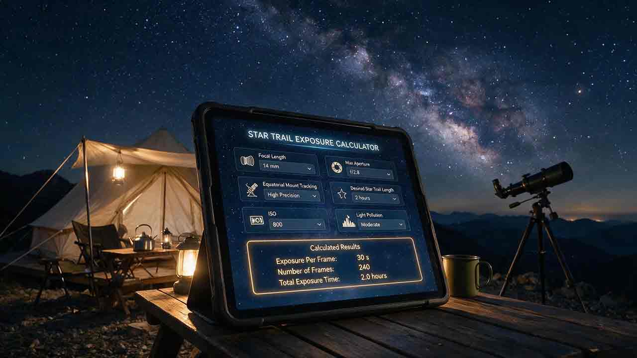
This guide explains how to calculate star-trail exposure time from Earth’s sidereal rotation, stellar declination, and local image scale. It distinguishes polar sweep, declination-adjusted sky-path length, projected pixel length, recorded sweep, missing sweep, and the full start-to-end span of a stacked sequence. Original tables compare trail lengths at several declinations, quantify one-second frame gaps at different image scales, and show how recorded time, gap time, duty cycle, and sequence sweep relate. The Trail–Frame–Sequence Check provides a practical framework for separating celestial geometry, per-frame reliability, and sequence continuity. Worked examples also address the celestial-pole edge case, local WCS-based pixel movement, frame-count limits, long-exposure noise reduction, and the difference between a single exposure and stacked frames. Readers can use the article to plan smoother trails, avoid misleading sequence calculations, and verify expected motion with native-resolution test images.
Camera Field of View Calculator
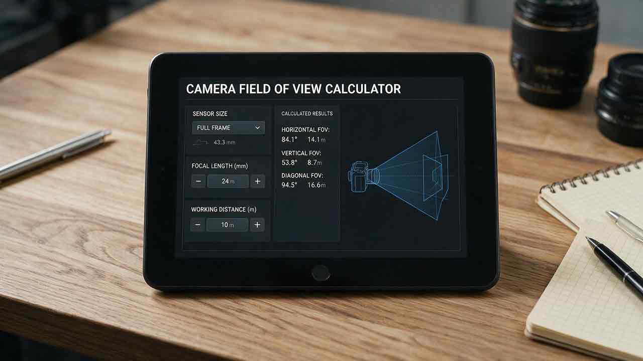
This guide explains how to calculate horizontal, vertical, and diagonal camera field of view from the recorded active sensor dimensions and effective focal length. It distinguishes physical focal length from crop-factor comparisons, shows why aspect ratio and target rotation affect framing, and provides independently calculated reference tables for common sensor sizes and focal lengths. The original Frame Envelope Check separates ideal frame geometry, the target envelope, and the usable frame retained after dithering, registration, distortion correction, and cropping. Worked examples demonstrate target occupancy, maximum permitted focal length, rotated bounding boxes, and mosaic panel counts with overlap. The article also explains radians versus degrees, crop and stabilization modes, focus breathing, rectilinear versus fisheye projection, and plate-solving verification through a celestial WCS. Readers can use the formulas, margin budget, troubleshooting table, and framing checklist to plan wide-field compositions, small-target imaging, or mosaics without treating a mathematical edge-to-edge fit as a guaranteed final frame.
Astrophotography Image Scale Calculator
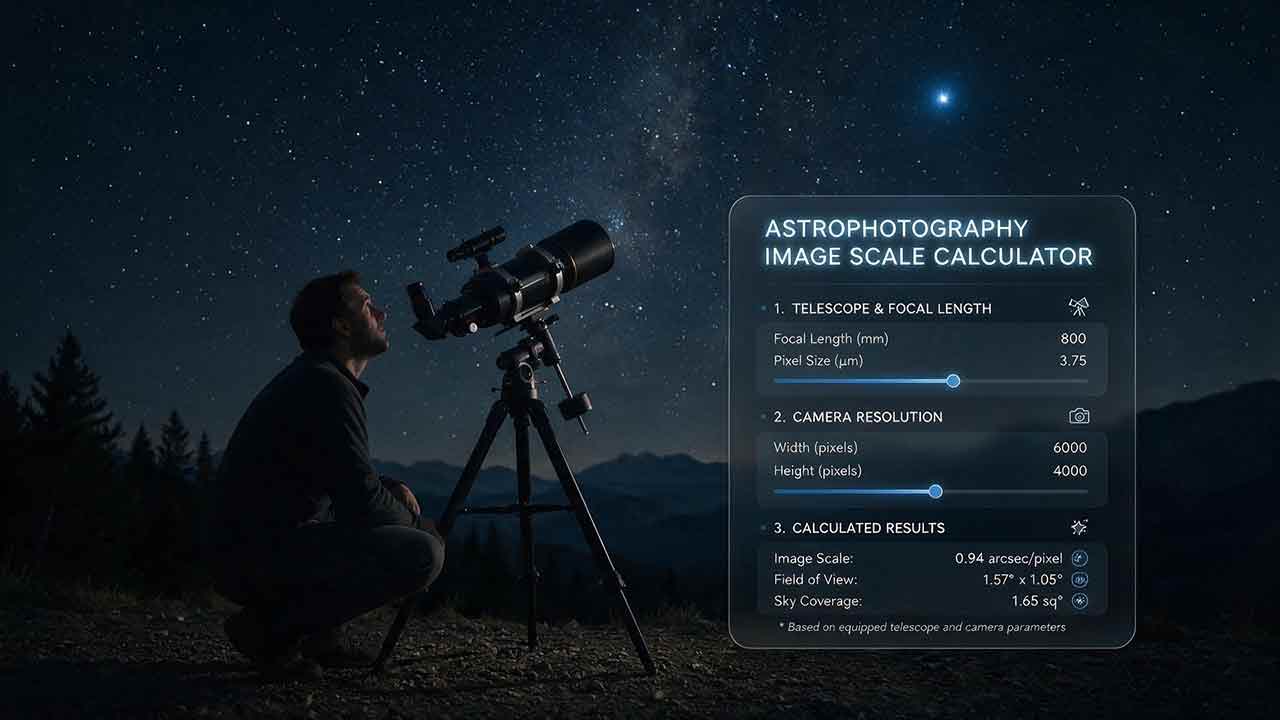
This guide explains how to calculate astrophotography image scale from camera pixel size and effective focal length, then interpret the result without confusing detector sampling with true optical resolution. It covers correct inputs, non-square pixels, reducers, amplifiers, binning, resampling, field of view, plate scale terminology, and WCS-based verification. Two original reference tables compare image scale across common pixel pitches and focal lengths and show how delivered stellar FWHM translates into pixels per FWHM. The original Scale–Quality–Target Check provides a practical decision framework for matching sampling to real image quality and target detail. Reproducible guidance explains how to measure representative FWHM from native-resolution data, diagnose discrepancies between calculated and plate-solved scale, and derive a local effective focal length. The article also distinguishes wide-field, small-target, lunar, planetary, photometric, and astrometric use cases while avoiding universal purchasing claims or unsupported equipment-testing conclusions.
Explore More Topics
Meteor Shower Visibility Calculator
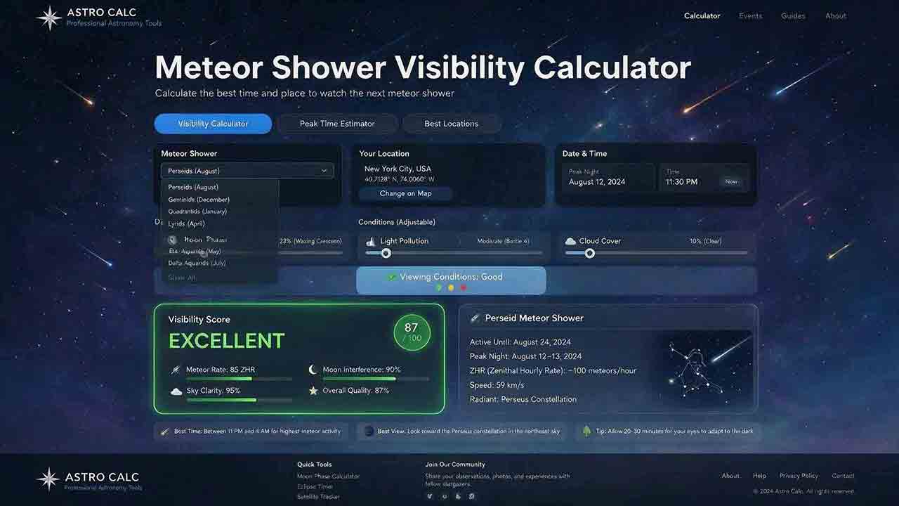
This guide explains how to use a meteor shower visibility calculator to identify a locally favorable observing window instead of relying only on a published peak time or Zenithal Hourly Rate. It covers activity periods, radiant altitude, astronomical darkness, Moon timing, weather, limiting magnitude, population index, and the distinction between named-shower members, sporadic meteors, and meteors from overlapping showers. The article introduces two original planning tools: the Five-Layer Meteor Test and the Meteor Opportunity Window, which calculates the overlap between activity, radiant, darkness, Moon, weather, and session constraints. A reproducible cross-midnight example compares illustrative 20° and 40° radiant thresholds, producing windows of 2 hours 20 minutes and 1 hour 40 minutes. Practical guidance addresses moonlight, viewing direction, dark adaptation, calculator disagreements, troubleshooting, and responsible site selection, supported by NASA, IMO, AMS, and U.S. Naval Observatory sources.

Planet Visibility Finder: Which Planets Can You See Tonight?
This guide explains how to use a planet visibility finder to decide which planets are realistically observable for a selected date, time, and location. It shows why an object being above the horizon does not guarantee visibility and explains the roles of altitude, azimuth, apparent magnitude, solar elongation, twilight, moonlight, weather, and local obstructions. Readers learn which planets are normally visible without a telescope, how Mercury and Venus differ from the outer planets, and why two finders may produce different results. The article introduces an original Four-Gate Visibility Test covering position, solar light, detectability, and site timing, plus a reproducible Useful Viewing Window calculation. A hypothetical example compares a 1-hour-26-minute naked-eye window with an 18-minute higher-altitude telescope window. Practical troubleshooting, safety guidance, and NASA, USNO, and JPL sources support the planning method.
Astronomical Twilight Calculator: When Does the Sky Become Dark?
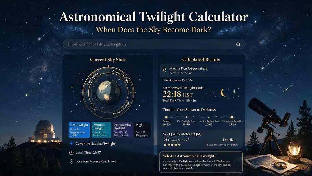
This guide explains how to use an astronomical twilight calculator to identify the end of evening astronomical twilight and the beginning of morning astronomical twilight for a selected date and location. It distinguishes sunset, civil dusk, nautical dusk, astronomical dusk, and the Sun-below-18° interval while clarifying that solar geometry does not guarantee a visibly dark sky. Readers learn how latitude, season, timezone, daylight-saving rules, moonlight, skyglow, clouds, haze, and high-latitude conditions affect practical planning. The article introduces two original tools: the Darkness Margin, which calculates how much of a session falls inside the Sun-below-18° interval, and a Task Threshold Matrix that matches observing goals to practical twilight stages. A worked cross-midnight example produces a 1-hour-48-minute dark interval. Troubleshooting guidance, planning checks, and authoritative USNO, NOAA, and National Park Service sources support the method.