Space Object Scale Comparison Tool

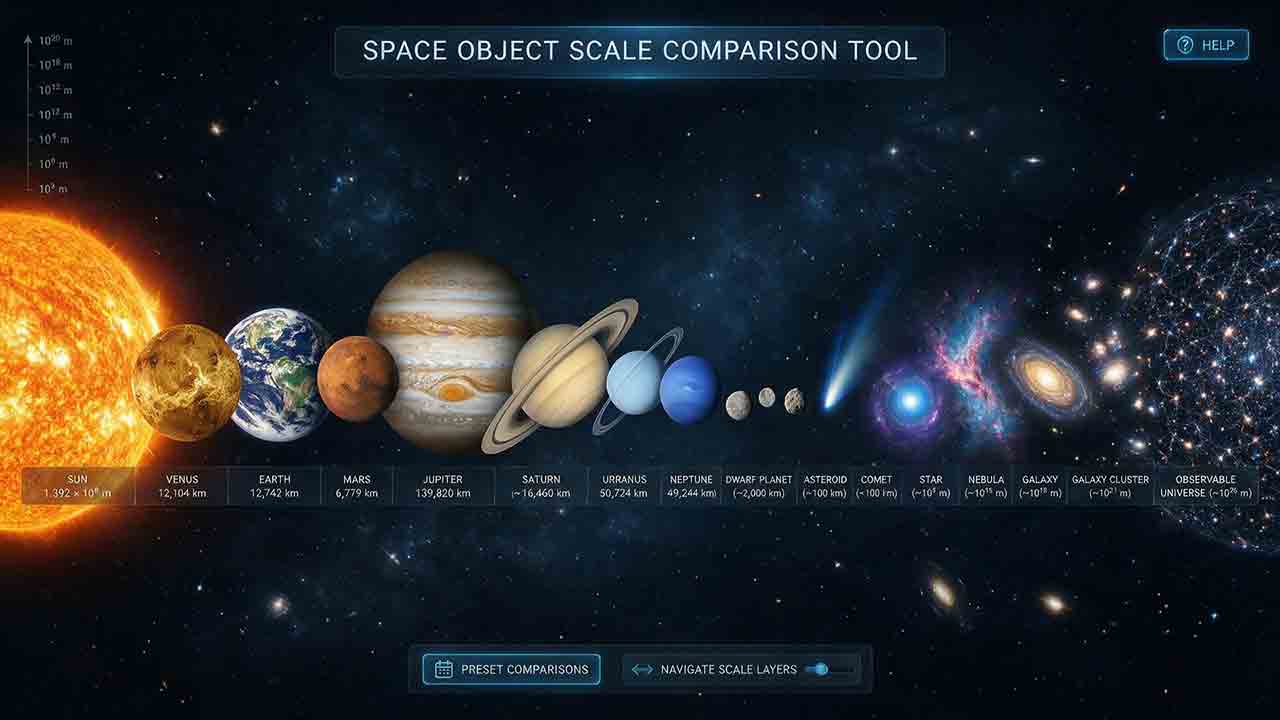
Space Object Scale Comparison Tool
A Space Object Scale Comparison Tool places selected planets, the Moon, dwarf planets, asteroid Bennu, and the Sun on one consistent linear scale. Choose two objects to compare, or assign one reference object a model diameter. The tool calculates diameter ratios and scaled model sizes from documented physical dimensions without mixing size, mass, orbital distance, or apparent angular width.
Key Takeaways
- The core comparison uses one-dimensional physical diameter or another explicitly labeled width.
- NASA/JPL equivalent-volume mean diameters provide a consistent default for nearly spherical planets and dwarf planets.
- The tool’s primary results are linear ratios and scaled diameters; area and volume relationships are separately labeled geometric derivations.
- Ring spans, comet comae, galaxy boundaries, and black-hole shadows are not interchangeable with solid-body diameters.
- A single linear graphic cannot faithfully display objects spanning millions in size ratio unless it uses zoom, insets, or separate panels.
This guide explains the tool’s verified preset range, the adopted size definitions, the scale formulas, the limits of derived area and volume ratios, and the checks needed to create an accurate comparison.
Calculation standard: The core preset comparison uses physical width. Planet and dwarf-planet values use twice the NASA/JPL equivalent-volume mean radius. The Moon uses twice its published mean radius. Bennu uses its approximate published equatorial width and is labeled accordingly. The Sun uses twice the IAU nominal solar radius of 695,700 km. Intermediate values are not rounded; displayed results reflect the precision of the source dimensions.
Quick formula guide
- Linear diameter ratio: (q=D_A/D_B)
- Reference percentage: (100q%)
- Scaled model size: (s_A=s_B(D_A/D_B))
- Reference-circle area ratio: (q^2)
- Reference-sphere volume ratio: (q^3)
- Scale factor: (k=s_{\text{reference}}/D_{\text{reference}})
What Does the Space Object Scale Comparison Tool Support?
The documented core tool compares a verified set of physical widths and calculates linear scale results.
Verified Preset Objects
The preset library documented on this page contains:
- Bennu
- Ceres
- Pluto
- the Moon
- Mercury
- Mars
- Venus
- Earth
- Neptune
- Uranus
- Saturn
- Jupiter
- the Sun
The tool does not claim built-in presets for:
- other asteroids or comets
- planetary ring systems
- stars other than the Sun
- exoplanets
- galaxies or nebulae
- black holes
Those objects can be discussed or added to a separate dataset only after a suitable physical boundary, dimension, source, and uncertainty have been identified.
Core Tool Outputs
| Core output | Meaning |
|---|---|
| Diameter ratio | Adopted width of object A divided by adopted width of object B |
| Reference percentage | Object A’s adopted width as a percentage of object B |
| Scaled model diameter | Model width after one object is assigned a reference size |
| Ordered lineup | Preset objects arranged by adopted physical width |
| Definition label | Mean diameter, nominal diameter, or approximate equatorial width |
| Source label | Authority supporting the adopted dimension |
The core outputs are linear.
The reference-circle area ratio and reference-sphere volume ratio discussed later are derived geometric interpretations. They should not be presented as direct measurements or as guaranteed interactive outputs unless the deployed interface explicitly includes them.
How Do You Use the Space Object Scale Comparison Tool?
Step 1: Choose the Comparison Mode
Use pair comparison to answer questions such as:
- How many times wider is Jupiter than Earth?
- What percentage of Earth’s diameter is the Moon?
- Is Uranus or Neptune larger by mean diameter?
Use scale-model mode when one object should represent a chosen model size.
Examples include:
- Earth = 1 cm
- Earth = 10 cm
- Jupiter = 1 m
- the Sun = 1 m
Step 2: Select the Reference Object
The reference object provides the denominator of the ratio.
If Earth is the reference:
[q\frac{D_{\text{object}}}{D_{\text{Earth}}}]
If Jupiter is the reference:
[q\frac{D_{\text{object}}}{D_{\text{Jupiter}}}]
Changing the reference reverses or otherwise changes the numerical ratio, but it does not change either object’s physical size.
Step 3: Enter the Model Diameter When Needed
In scale-model mode, assign the reference object a positive finite model diameter.
For example:
[s_{\text{Earth}}10\ \text{cm}]
Every selected object is then multiplied by the same scale factor.
Step 4: Read the Definition Label
Do not compare numbers until their meanings are clear.
The presets on this page use:
- equivalent-volume mean diameter for planets and dwarf planets
- mean diameter for the Moon
- approximate equatorial width for Bennu
- nominal diameter for the Sun
These definitions are visible because they are not physically identical.
Step 5: Choose an Appropriate Display
Use:
- one linear lineup for objects with a manageable size range
- separate linear panels for very different size groups
- enlarged insets for tiny objects
- a logarithmic chart for orders-of-magnitude comparison
- a ratio table when numerical accuracy matters most
A logarithmic chart is useful for overview, but it is not a literal side-by-side scale model.
Step 6: Keep Size and Distance Separate
This tool compares object dimensions.
It does not automatically place orbital distances on the same scale. For orbital spacing, use the Solar System Scale Calculator. For apparent width from an observer’s location, use the Angular Size Calculator.
How Does the Linear Scale Calculation Work?
Let:
- (D_A) be the adopted real diameter of object A
- (D_B) be the adopted real diameter of reference object B
- (s_B) be the selected model diameter of object B
- (s_A) be the calculated model diameter of object A
The linear ratio is:
[q\frac{D_A}{D_B}]
The percentage of the reference size is:
[P100\frac{D_A}{D_B}]
The scaled model diameter is:
[s_As_B\frac{D_A}{D_B}]
The physical dimensions must be expressed in compatible linear units before division.
Scale-Factor Form
The scale factor is:
[k\frac{s_B}{D_B}]
Every model dimension is then:
[s_ikD_i]
Using one retained scale factor is safer than independently rounding each object ratio.
Worked Example: Earth as a 10 cm Model
NASA/JPL gives Earth an equivalent-volume mean radius of:
[6{,}371.0084\ \text{km}]
The adopted mean diameter is:
[D_E2\times6{,}371.0084]
[D_E12{,}742.0168\ \text{km}]
Suppose the model Earth is:
[s_E10\ \text{cm}]
The Moon’s adopted mean diameter is:
[D_M2\times1{,}737.4]
[D_M3{,}474.8\ \text{km}]
The Moon model diameter is:
[s_M10\frac{3{,}474.8}{12{,}742.0168}]
[s_M\approx2.727\ \text{cm}]
The same scale factor must be used for Jupiter, the Sun, Bennu, and every other selected preset.
Which Diameter Definition Should You Use?
The strongest definition is the one that matches the comparison question.
| Object or purpose | Recommended dimension | Advantage | Limitation |
|---|---|---|---|
| Nearly spherical planet | Equivalent-volume mean diameter | Consistent overall comparison | Hides equatorial bulging |
| Rapidly rotating planet | Equatorial and polar diameters | Shows oblateness | Requires two dimensions |
| Large spherical moon | Mean diameter | Compatible with planet presets | Local topography is omitted |
| Irregular asteroid | Axis dimensions or labeled width | Preserves shape information | One number cannot show the full shape |
| Volume comparison | Equivalent-volume diameter | Supports a meaningful sphere-volume comparison | Does not preserve the visible outline |
| Ringed planet | Body diameter and ring span separately | Prevents body/ring confusion | Requires separate layers |
| Comet | Nucleus dimensions | Represents the persistent solid body | Excludes changing coma and tail |
| Star | Cited photospheric or nominal diameter | Uses an identified stellar convention | A star has no solid surface |
| Exoplanet | Published modeled or transit radius | Uses cataloged observational results | Depends on model and stellar parameters |
| Diffuse object | Major and minor axes at a stated boundary | Makes the observational definition explicit | Boundary can vary by survey or wavelength |
Why Use Equivalent-Volume Mean Diameter for Planets?
The NASA/JPL Planetary Physical Parameters table defines mean radius as the radius of a sphere with the same volume as the planet.
The corresponding mean diameter is:
[D_{\text{mean}}2R_{\text{mean}}]
This gives one reproducible width while preserving volume through the equivalent-sphere definition.
It does not imply that the actual planet is perfectly spherical or that every projected view has the same diameter.
Which Reference Dimensions Are Used?
| Object | Adopted dimension | Definition | Ratio to Earth |
|---|---|---|---|
| Bennu | 0.492 km | Approximate equatorial width | 0.00003861 |
| Ceres | 939.4 km | Equivalent-volume mean diameter | 0.07372 |
| Pluto | 2,376.6 km | Mean diameter | 0.1865 |
| Moon | 3,474.8 km | Mean diameter | 0.2727 |
| Mercury | 4,878.8 km | Equivalent-volume mean diameter | 0.3829 |
| Mars | 6,779.0 km | Equivalent-volume mean diameter | 0.5320 |
| Venus | 12,103.6 km | Mean diameter | 0.9499 |
| Earth | 12,742.0168 km | Equivalent-volume mean diameter | 1.0000 |
| Neptune | 49,244 km | Equivalent-volume mean diameter | 3.865 |
| Uranus | 50,724 km | Equivalent-volume mean diameter | 3.981 |
| Saturn | 116,464 km | Equivalent-volume mean diameter | 9.140 |
| Jupiter | 139,822 km | Equivalent-volume mean diameter | 10.97 |
| Sun | 1,391,400 km | Twice the nominal solar radius | 109.2 |
Planet and dwarf-planet dimensions are derived from the NASA/JPL planetary mean-radius table.
The Moon uses the mean radius in the NASA/JPL Planetary Satellite Physical Parameters table.
Bennu’s value follows the NASA Bennu facts page, which describes an approximate equatorial width rather than a perfect spherical diameter.
The Sun uses the IAU nominal solar radius:
[\mathcal{R}_{\odot}^{N}695{,}700\ \text{km}]
The nominal solar diameter is therefore:
[2\mathcal{R}_{\odot}^{N}1{,}391{,}400\ \text{km}]
The nominal radius is a standardized conversion constant. It is not a claim that the Sun has a perfectly sharp, unchanging physical edge.
Why Is Uranus Larger Than Neptune in This Table?
Uranus has the larger NASA/JPL equivalent-volume mean radius:
[R_{\text{Uranus}}25{,}362\ \text{km}]
[R_{\text{Neptune}}24{,}622\ \text{km}]
Therefore:
[D_{\text{Uranus}}>D_{\text{Neptune}}]
by the adopted mean-diameter definition.
Neptune is more massive than Uranus. The ranking changes because size and mass are different physical quantities.
A heading such as “largest planets” should therefore state whether it means diameter, volume, mass, or another property.
What Do the (q^2) and (q^3) Comparisons Mean?
The primary result is the linear ratio:
[q\frac{D_A}{D_B}]
The squared and cubed values are model-derived comparisons, not additional measured dimensions.
Reference-Circle Area Ratio
Define a circle for each object whose diameter equals the adopted comparison diameter.
The area ratio of those reference circles is:
[\frac{A_{A,\text{circle}}}{A_{B,\text{circle}}}q^2]
This should be labeled:
Reference-circle area ratio
It represents actual projected-area ratio only when the selected objects can reasonably be represented by circular projections using the adopted diameters.
It is not automatically the actual projected area of:
- an irregular asteroid
- an inclined disk
- a ring system
- a visibly oblate planet at every orientation
- a diffuse object with an uncertain boundary
Reference-Sphere Volume Ratio
Define a sphere for each object whose diameter equals the adopted comparison diameter.
The ratio is:
[\frac{V_{A,\text{sphere}}}{V_{B,\text{sphere}}}q^3]
This should be labeled:
Reference-sphere volume ratio
When both adopted values are equivalent-volume diameters, (q^3) also gives the physical volume ratio by definition.
When the input is a maximum width, ring span, nominal stellar radius, or another non-volume-equivalent dimension, (q^3) is only a reference-sphere model.
Core–Derived–Custom Output Ladder
Use this three-level rule:
- Core output: sourced linear diameter ratio and model size.
- Derived output: reference-circle (q^2) or reference-sphere (q^3), with assumptions stated.
- Custom scientific interpretation: actual area, volume, or boundary analysis using object-specific geometry and data.
This distinction prevents a correct exponent from being attached to the wrong physical meaning.
Derived Geometric Comparison Examples
| Object relative to Earth | Diameter ratio | Reference-circle area ratio | Reference-sphere volume ratio |
|---|---|---|---|
| Moon | 0.2727 | 0.07437 | 0.02028 |
| Mars | 0.5320 | 0.2830 | 0.1506 |
| Jupiter | 10.9733 | 120.4 | 1,321 |
| Sun | 109.198 | 11,924 | (1.30\times10^6) |
For the Moon, Mars, Jupiter, and Earth, the adopted mean diameters are based on mean or equivalent-volume radii. The cubed ratios therefore have a clear equivalent-sphere interpretation.
For the Sun, the final column is specifically a nominal-sphere volume ratio based on the IAU nominal solar radius.
The values do not represent mass ratios. Objects with different densities can have very different mass and volume rankings.
What Does an Earth-at-10-Centimeters Model Look Like?
The following table assigns Earth a model diameter of exactly 10 cm.
| Object | Scaled model diameter |
|---|---|
| Bennu | 0.00386 mm |
| Ceres | 7.37 mm |
| Pluto | 18.7 mm |
| Moon | 27.3 mm |
| Mercury | 38.3 mm |
| Mars | 53.2 mm |
| Venus | 95.0 mm |
| Earth | 100 mm |
| Neptune | 386 mm |
| Uranus | 398 mm |
| Saturn | 914 mm |
| Jupiter | 1.097 m |
| Sun | 10.92 m |
Bennu’s result uses its approximate 492 m equatorial width. It is not labeled as an equivalent-volume mean diameter.
This model exposes a practical conflict: a scale large enough to make small planets easy to see makes the Sun more than ten meters wide.
What Is the Scale-Span Problem?
The scale span is the ratio between the largest and smallest selected physical widths:
[S_{\text{span}}\frac{D_{\max}}{D_{\min}}]
Using the nominal solar diameter and Bennu’s approximate equatorial width:
[S_{\text{span}}\frac{1{,}391{,}400\ \text{km}}{0.492\ \text{km}}]
[S_{\text{span}}\approx2.83\times10^6]
The order-of-magnitude span is:
[\log_{10}(S_{\text{span}})\approx6.45]
Suppose the Sun is rendered 1,200 pixels wide. Bennu’s proportional width would be:
[\frac{1{,}200}{2.83\times10^6}]
[\approx0.00042\ \text{pixel}]
That value is mathematically valid but impossible to display as a visible feature.
The Definition–Ratio–Resolution Framework
A trustworthy comparison should pass three checks:
- Definition: Do the selected dimensions describe comparable boundaries?
- Ratio: Is the result linear, reference-circle area, or reference-sphere volume?
- Resolution: Can the smallest object remain visible at the chosen display size?
This framework separates correct arithmetic from honest visualization.
Which Display Method Should You Use?
| Display method | Best use | Main advantage | Main limitation |
|---|---|---|---|
| Single linear lineup | Objects within a limited size range | Direct visual proportions | Small objects disappear |
| Enlarged inset | One or two tiny objects | Preserves local detail | Inset does not share the main display scale |
| Separate linear panels | Planets, dwarf planets, and small bodies | Keeps each group readable | Panels use different scales |
| Logarithmic chart | Several orders of magnitude | Keeps all objects visible | Bar lengths are not literal diameters |
| Ratio table | Exact comparison and auditing | Compact and precise | Less visually immediate |
| Physical model | Classroom or exhibition | Tangible and memorable | Large models require space |
| Interactive zoom | Digital exploration | Can retain one mathematical scale | Requires visible scale indicators |
Practical Display Rule
A single linear panel works best when the largest selected object is no more than a few dozen times wider than the smallest.
For a much broader range, use:
- a separate inset
- grouped linear panels
- interactive zoom
- a logarithmic overview
- a numerical table beside the visualization
Every inset or alternate scale should be labeled.
How Should Non-Preset Objects Be Handled?
The following categories are outside the verified preset library documented on this page. They require an object-specific dimension and source before being added.
| Object type | Dimension to identify | Required warning |
|---|---|---|
| Irregular asteroid | Three axes, longest width, or equivalent-volume diameter | One width does not preserve shape |
| Planetary rings | Planetary body diameter and selected ring boundary separately | Rings are not part of the planet’s body diameter |
| Comet | Nucleus size, coma size, or tail length | These structures have different physical meanings |
| Other star | Photospheric or model radius | A star has no hard solid edge |
| Exoplanet | Published radius and uncertainty | Value depends on observations and stellar modeling |
| Galaxy or nebula | Major/minor axes at a stated survey boundary | Diffuse extent can depend on wavelength and threshold |
| Black hole | Event horizon, shadow, or accretion structure | These boundaries are not interchangeable |
Irregular Asteroids
For an ellipsoid with full axis lengths:
[a\times b\times c]
an equivalent-volume diameter can be defined as:
[D_{\text{eq}}(abc)^{1/3}]
This preserves the ellipsoid’s volume in a sphere model.
The original axes should still be retained when the actual outline matters.
The NASA/JPL Small-Body Database provides physical parameters and references when such measurements are available.
Planetary Ring Systems
A ring span must be displayed separately from the planet’s body diameter.
NASA explains that Saturn’s visible ring system extends far beyond the planet and includes boundaries that differ between the bright main rings, the F ring, the diffuse E ring, and the distant Phoebe ring. See NASA Saturn Facts and the Cassini ring overview.
A responsible scale graphic should identify exactly which ring boundary it uses.
Comets
NASA distinguishes a comet’s persistent nucleus from its changing coma and tails.
The NASA Comet Facts page explains that the nucleus may be only a few kilometers wide while the coma can extend hundreds of thousands of kilometers.
Use the nucleus for a solid-body comparison. A coma or tail can be shown only as a separately labeled temporary structure.
Stars Other Than the Sun
A stellar radius should identify the photospheric or model convention used.
Do not assume that every cataloged stellar radius represents a sharp physical surface. The Sun preset uses the nominal solar radius only as a standardized conversion value.
Exoplanets
The NASA Exoplanet Archive parameter documentation identifies planet-radius values, units, uncertainties, limits, and literature references.
Before adding an exoplanet, confirm:
- the selected parameter set
- whether the radius is measured or calculated
- its uncertainty
- whether it is an upper limit
- the adopted Earth-radius or Jupiter-radius convention
Galaxies and Nebulae
Galaxies and nebulae do not usually have a solid edge comparable to a planetary surface.
A custom entry should identify:
- major and minor axes
- physical or angular units
- observing wavelength
- survey or instrument
- distance used for physical-size conversion
- brightness threshold or contour when relevant
NASA describes nebulae as diffuse clouds of gas and dust in its Hubble nebula guide.
These diffuse objects are better handled by a dedicated observational-size dataset than by the core planet preset list.
Black Holes
A black-hole entry must specify the selected boundary.
NASA distinguishes the event horizon, event-horizon shadow, photon structures, and accretion disk in its black-hole anatomy guide.
A shadow diameter is not the same as an event-horizon diameter, and an accretion disk can extend much farther than either. The core tool therefore does not include a generic “black-hole diameter” preset.
How Is Physical Size Different From Apparent Size?
Physical size is an intrinsic length. Apparent size is the angle an object spans from an observer’s location.
A physically smaller nearby object can appear larger than a more distant object with a greater physical diameter.
For a centered symmetric width:
[\theta2\arctan\left(\frac{D}{2L}\right)]
where:
- (D) is physical width
- (L) is the perpendicular observer distance
- (\theta) is full angular width
Use the Angular Size Calculator when the question concerns how large an object appears.
The core scale comparison intentionally removes observer distance from the diameter ratio.
Why Are Object Sizes and Orbital Distances Usually Shown Separately?
Object diameter and orbital spacing differ by many orders of magnitude.
If Earth were 1 cm wide, one astronomical unit would scale to:
[1\ \text{cm}\timesfrac{149{,}597{,}870.7\ \text{km}}{12{,}742.0168\ \text{km}}]
[\approx117.4\ \text{m}]
A row that makes Earth 1 cm wide while placing the Sun only a few centimeters away cannot have both sizes and distances to scale.
A visualization should state one of the following:
- sizes to scale; distances not to scale
- sizes and distances both to scale
- logarithmic distance display
- schematic layout
How Does Source Uncertainty Affect a Size Ratio?
For:
[q\frac{D_A}{D_B}]
with approximately independent uncertainties:
[\left(\frac{\sigma_q}{q}\right)^2\approx\left(\frac{\sigma_A}{D_A}\right)^2+\left(\frac{\sigma_B}{D_B}\right)^2]
Example
Suppose:
[D_A1{,}000\pm30\ \text{km}]
and:
[D_B500\pm10\ \text{km}]
The central ratio is:
[q2.0]
The approximate fractional uncertainty is:
[\frac{\sigma_q}{q}\approx\sqrt{0.03^2+0.02^2}]
[\approx0.036]
Therefore:
[q\approx2.00\pm0.07]
A result such as 2.000000 would imply unsupported physical precision.
Uncertainty in a Scaled Model
When the model reference size is treated as exact:
[s_AkD_A]
the relative source uncertainty is unchanged:
[\frac{\sigma_{s_A}}{s_A}\frac{\sigma_{D_A}}{D_A}]
The scale model does not make the source dimension more accurate.
Which Values Can Verify the Tool?
| Test | Expected result |
|---|---|
| Earth compared with itself | exactly 1 |
| Moon divided by Earth mean diameter | approximately 0.272704 |
| Mars divided by Earth mean diameter | approximately 0.532019 |
| Venus divided by Earth mean diameter | approximately 0.949897 |
| Jupiter divided by Earth mean diameter | approximately 10.9733 |
| Sun nominal diameter divided by Earth mean diameter | approximately 109.198 |
| Earth model 10 cm → Moon | approximately 2.727 cm |
| Earth model 10 cm → Jupiter | approximately 109.7 cm |
| Earth model 10 cm → Sun | approximately 10.92 m |
| Doubling the model reference size | doubles every model diameter |
| Changing all real-size units consistently | leaves every ratio unchanged |
Extended values are intended for implementation testing. Displayed values should be rounded according to source precision and the practical resolution of the model or graphic.
Ratio Reversal Test
If:
[q_{AB}\frac{D_A}{D_B}]
then:
[q_{BA}\frac{D_B}{D_A}]
and:
[q_{AB}q_{BA}1]
For Jupiter and Earth:
[q_{JE}\approx10.9733][q_{EJ}\approx0.091130]
Their unrounded product should return 1 within numerical precision.
Model Back-Calculation Test
From:
[s_As_B\frac{D_A}{D_B}]
the model must preserve:
[\frac{s_A}{s_B}\frac{D_A}{D_B}]
A failure indicates a unit mismatch, reversed ratio, inconsistent definition, or premature rounding.
Reference-Derivation Test
When a reference-circle area ratio is shown:
[A_{\text{ratio}}q^2]
When a reference-sphere volume ratio is shown:
[V_{\text{ratio}}q^3]
The interface or result label must not shorten these to “area” or “volume” without preserving the reference-circle or reference-sphere qualification.
Common Scale-Comparison Errors and Troubleshooting
| Problem | Likely cause | What to check |
|---|---|---|
| Every result is off by a factor of two | Radius was entered as diameter | Confirm whether the value is (R) or (D=2R) |
| Uranus and Neptune appear in the wrong order | Mean and equatorial diameters were mixed | Use one stated convention |
| Jupiter volume comparison looks too small | Linear ratio was mistaken for volume ratio | Use the reference-sphere (q^3) value |
| (q^2) is labeled as actual projected area | Geometric assumptions were omitted | Use the reference-circle label |
| (q^3) is labeled as actual volume | Diameter was not volume-equivalent | Use the reference-sphere label |
| Mass is presented as size | Physical quantities were confused | Label diameter, mass, and volume separately |
| Saturn appears excessively large | Ring span replaced body diameter | Show rings separately |
| Bennu appears spherical | Equatorial width was treated as a complete shape | Retain its approximate-width label |
| A comet dominates the lineup | Coma or tail replaced nucleus size | Identify the selected component |
| Tiny objects disappear | Scale span exceeds display resolution | Add an inset, panel, or zoom |
| Planet spacing looks realistic but is not | Orbital distances are schematic | Add a distance-scale label |
| Exoplanet has too many decimals | Catalog uncertainty was ignored | Show uncertainty and source |
| Star size differs by source | Different stellar radius conventions were mixed | Compare the definitions |
| Diffuse-object size differs by wavelength | Different boundaries were used | State survey and wavelength |
| Custom value gives no result | Input validation failed | Require a positive finite physical size |
Space Object Scale Audit Checklist
Before publishing or relying on a comparison, confirm:
- Every core value is a physical width rather than mass, distance, or angular size.
- Radius and diameter are not mixed.
- Mean, equatorial, nominal, and approximate widths are labeled.
- Only the documented objects are described as built-in presets.
- The same linear units are used internally.
- Linear ratio and scaled diameter remain the primary outputs.
- (q^2) is labeled as a reference-circle area ratio.
- (q^3) is labeled as a reference-sphere volume ratio.
- Equivalent-volume claims use compatible mean diameters.
- Rings, comae, tails, atmospheres, and halos are separate structures.
- Irregular objects retain axis or width information.
- Small objects remain visible or receive a labeled inset.
- Linear and logarithmic displays are distinguished.
- Object size and orbital spacing are not silently mixed.
- Source uncertainty controls display precision.
- Nominal constants are identified as conventions.
- Derived ratios are not described as direct measurements.
- Non-preset objects include an appropriate source and boundary definition.
- Results are not presented as mission-navigation or engineering data.
Practical Conclusion
Use the Space Object Scale Comparison Tool to compare verified physical widths on one consistent linear scale. The core preset library covers Bennu, Ceres, Pluto, the Moon, the eight planets, and the Sun. Its strongest outputs are diameter ratio, percentage of the reference, and scaled model diameter.
Educators can assign Earth a convenient classroom size. Designers should use insets or separate panels when the scale span makes small objects invisible. Technical writers should retain the source definition and uncertainty. Rings, comets, other stars, exoplanets, diffuse objects, and black holes require a custom boundary and should not be presented as ordinary planet-diameter presets.
Scope notice: This tool is intended for education, visualization, preliminary comparison, and general scientific reference. Detailed shape modeling, instrument analysis, spacecraft navigation, and mission planning require validated object-specific datasets and specialist methods.
Related Space Distance and Scale Tools
- Astronomical Distance Converter — convert physical widths and model dimensions into compatible units.
- Angular Size Calculator — calculate how large an object appears from a known observer distance.
- Planet Weight Calculator — compare mass and gravitational force without confusing them with size.
- Planet Distance Calculator — obtain or compare observer-to-planet distances.
- Solar System Scale Calculator — model both object dimensions and orbital spacing with a stated scale.
Frequently Asked Questions
How Many Earths Fit Across Jupiter?
Using the adopted NASA/JPL mean diameters:
[\frac{D_J}{D_E}\approx10.97]
Jupiter is therefore about 11 Earth mean diameters wide.
How Many Earth Volumes Fit Inside Jupiter?
The reference-sphere ratio based on the adopted mean diameters is:
[\left(\frac{D_J}{D_E}\right)^3\approx1{,}321]
Because the adopted planetary values are equivalent-volume mean diameters, this also represents their approximate physical volume ratio. It is not a mass ratio.
Is Uranus Larger Than Neptune?
Uranus has the larger NASA/JPL equivalent-volume mean diameter.
Neptune is more massive, so the answer changes when “larger” refers to mass rather than physical width.
Should Saturn’s Rings Count Toward Its Size?
Only when the comparison explicitly concerns a selected ring boundary.
For a planet-body comparison, use Saturn’s mean diameter and display the rings as a separate labeled structure.
Why Does Bennu Disappear Beside the Sun?
The adopted Sun-to-Bennu width ratio is approximately (2.83\times10^6).
A normal screen or printed page cannot represent that span faithfully on one linear panel, so Bennu requires an inset, separate panel, or interactive zoom.
Is Physical Diameter the Same as Angular Size?
No. Physical diameter is an intrinsic length.
Angular size depends on both physical width and observer distance. Use the Angular Size Calculator when the question concerns apparent size.
Sources
NASA/JPL Solar System Dynamics — Planetary Physical Parameters
Provides equatorial and equivalent-volume mean radii for planets and selected dwarf planets and defines the radius conventions. Accessed August 1, 2026.NASA/JPL Solar System Dynamics — Planetary Satellite Physical Parameters
Provides mean radii and supporting references for the Moon and other planetary satellites. Accessed August 1, 2026.International Astronomical Union — Nominal Units for Stellar and Planetary Astronomy
Provides access to IAU Resolution B3 and nominal solar and planetary conversion constants. Accessed August 1, 2026.NASA Science — Universe Glossary
Gives the nominal solar radius used as a stellar-size conversion unit. Accessed August 1, 2026.NASA Science — Bennu Facts
Describes Bennu’s approximate equatorial width and irregular top-like shape. Accessed August 1, 2026.NASA/JPL Solar System Dynamics — Small-Body Database Lookup
Provides available dimensions, physical parameters, uncertainties, and references for asteroids and comets. Accessed August 1, 2026.NASA Science — Saturn Facts
Describes Saturn’s rings and the large difference between planetary-body diameter and ring-system extent. Accessed August 1, 2026.NASA Cassini Mission — Rings
Explains the structure, particles, and diffuse boundaries of Saturn’s ring system. Accessed August 1, 2026.NASA Science — Comet Facts
Distinguishes a comet’s persistent nucleus from its changing coma and tails. Accessed August 1, 2026.NASA Exoplanet Archive — Planetary Systems Column Definitions
Defines planet-radius values, units, uncertainties, limits, and source-reference fields. Accessed August 1, 2026.NASA Exoplanet Archive — Composite Parameter Calculations
Explains how selected catalog parameters may be calculated when a direct empirical value is unavailable. Accessed August 1, 2026.NASA Hubble — Nebulae
Describes nebulae as diffuse gas-and-dust structures rather than solid objects with one universal edge. Accessed August 1, 2026.NASA Science — Anatomy of a Black Hole
Distinguishes the event horizon, event-horizon shadow, photon structures, and accretion disk. Accessed August 1, 2026.NASA Science — Planet Sizes and Locations
Provides an accessible distinction between planetary dimensions and orbital locations. Accessed August 1, 2026.
More from Space Distance & Scale Tools
Planet Weight Calculator
This guide explains how a planet weight calculator separates unchanged mass from gravitational force and standard-Earth force equivalents. It shows how to calculate weight with W = mg, interpret kilograms, pound-mass, newtons, pound-force, kg-equivalent, and lb-equivalent, and understand why local scale readings depend on instrument calibration. Sourced gravity presets cover the eight planets, the Moon, and Pluto, with clear warnings for giant planets that have no solid surface. Worked examples, verification values, altitude limits, custom-planet formulas, uncertainty propagation, and the original Reference–Instrument–Support Check help readers evaluate results without confusing force, mass, apparent weight, or reference gravity. The article also explains free fall, reference radii, Pluto data differences, and when a body-specific gravity model is required.
Angular Size Calculator
This guide explains how to calculate angular size, physical size, or distance using projected-width, spherical-limb, and small-angle geometry. It defines the correct distance for a flat projected width, distinguishes center distance for a spherical body, and shows when the small-angle approximation is accurate enough. Readers can verify calculator output with independent test values, a back-calculation check, worked Moon and deep-sky examples, and a reproducible approximation-error table. The article also covers radians, degrees, arcminutes, arcseconds, orientation, field of view, pixel coverage, uncertainty, catalog size differences, and angular-diameter distance in cosmology. Its Geometry–Quantity–Scale check and audit checklist help prevent radius-versus-diameter mistakes, mixed units, incorrect distance inputs, and confusion between angular size, resolution, and field of view.
Astronomical Distance Converter
This article explains how to convert astronomical distances among meters, kilometers, international miles, astronomical units, light-seconds, light-minutes, light-hours, light-days, light-years, parsecs, kiloparsecs, megaparsecs, and gigaparsecs. It presents the common-base conversion formula, authoritative unit definitions, implementation test values, and a back-conversion check for verifying calculator accuracy. Readers also learn how to choose an appropriate unit with the Scale–Purpose–Precision framework, preserve significant figures, propagate uncertainty, and distinguish exact conversion constants from uncertain astronomical measurements. Worked examples cover Earth–Moon, stellar, and galactic scales, while the troubleshooting table addresses common prefix, rounding, and unit errors. The guide also clarifies why unit conversion alone cannot determine a planet’s current distance or turn redshift directly into a cosmological distance.
Explore More Topics
Astrophotography Storage Calculator
This guide explains how to estimate storage for astrophotography capture, processing, and backup without relying on misleading megapixel shortcuts. It compares measured-file, uncompressed-array, and bitrate methods; distinguishes mean, median, high-percentile, and maximum file-size statistics; and explains decimal versus binary storage units. Readers learn how FITS headers, padding, HDUs, RAW compression, calibration frames, RGB conversion, drizzle, mosaics, caches, and temporary files affect project size. Original planning tools include the Four-Bucket Storage Ledger, the Capture–Process–Protect Check, and a clearly defined storage expansion ratio. Worked examples show how to calculate peak logical data, project-relative headroom, complete-copy footprint, media count, write rate, and transfer time. The article also covers integrity verification, backup limitations, retention decisions, and troubleshooting. It is designed to help astrophotographers build realistic capacity plans for single sessions, multi-night projects, planetary video, star trails, and long-term archives.
Star Trail Exposure Calculator
This guide explains how to calculate star-trail exposure time from Earth’s sidereal rotation, stellar declination, and local image scale. It distinguishes polar sweep, declination-adjusted sky-path length, projected pixel length, recorded sweep, missing sweep, and the full start-to-end span of a stacked sequence. Original tables compare trail lengths at several declinations, quantify one-second frame gaps at different image scales, and show how recorded time, gap time, duty cycle, and sequence sweep relate. The Trail–Frame–Sequence Check provides a practical framework for separating celestial geometry, per-frame reliability, and sequence continuity. Worked examples also address the celestial-pole edge case, local WCS-based pixel movement, frame-count limits, long-exposure noise reduction, and the difference between a single exposure and stacked frames. Readers can use the article to plan smoother trails, avoid misleading sequence calculations, and verify expected motion with native-resolution test images.
Camera Field of View Calculator
This guide explains how to calculate horizontal, vertical, and diagonal camera field of view from the recorded active sensor dimensions and effective focal length. It distinguishes physical focal length from crop-factor comparisons, shows why aspect ratio and target rotation affect framing, and provides independently calculated reference tables for common sensor sizes and focal lengths. The original Frame Envelope Check separates ideal frame geometry, the target envelope, and the usable frame retained after dithering, registration, distortion correction, and cropping. Worked examples demonstrate target occupancy, maximum permitted focal length, rotated bounding boxes, and mosaic panel counts with overlap. The article also explains radians versus degrees, crop and stabilization modes, focus breathing, rectilinear versus fisheye projection, and plate-solving verification through a celestial WCS. Readers can use the formulas, margin budget, troubleshooting table, and framing checklist to plan wide-field compositions, small-target imaging, or mosaics without treating a mathematical edge-to-edge fit as a guaranteed final frame.